GrUMPy 0.9.0

Now with Python 3 support!

Graphics for Understanding Mathematical Programming in Python (GrUMPy) is a Python library for visualizing various aspects of mathematical programming, including visualizations of the branch-and process, branch-and-bound trees, polyhedra, cutting plane methods, etc. The goal is clarity in implementation rather than efficiency. Most methods have an accompanying visualization and are thus appropriate for use in the classroom.

Documentation for the API is here:

https://tkralphs.github.io/GrUMPy

Pypi download page is here:

https://pypi.python.org/pypi/coinor.grumpy

See below for brief documentation of usage

##Installation Notes

To install, do:

pip install coinor.grumpy

1. GrUMPy depends on GiMPy, which will be automatically installed as part of the setup. However, in order for GiMPy to visualize the branch-and-bound tree, it's necessary to install GraphViz and choose one of these additional methods for display:

• Recommended: xdot 0.6.
  • Install with pip install xdot==0.6
  • Call set_display_mode('xdot') Note that xdot 0.6 depends on PyGtk (see below for platform-specific installation instructions for installing).
• Python Imaging Library and call set_display_mode('PIL')
• Pygame and call set_display_mode('pygame')
• Call set_display_mode('file') to just write files to disk that have to then be opened manually.

It is also possible to typeset labels in LaTex and to output the graph in LaTex format using dot2tex (Warning: recent versions of dot2tex have not perfectly, your mileage may vary). After installing dot2tex, this can be done by simply calling the method write(basename='fileName', format='dot'), and then doing dot2tex --tmath fileName.dot or by calling set_display_mode('dot2tex') and then display() as usual. At the moment, the latter only seems to work with version 2.9.0dev available here. For the former method, just using easy_install dot2tex should work fine.

1. GrUMPy also creates some visualizations with gnuplot. For tips on installing gnuplot, see below.
2. GrUMPy can also visualize 2D polyhedra with the installation of pypolyhedron, which can be install with pip install pypolyhedron

Additional Notes for Windows Installation

• To install Graphviz, download the installer here. Important: after installing, you must manually add the graphviz bin directory (usually C:\Program Files (x86)\Graphviz2.38\bin) to your PATH
• If you want to use xdot, there are some more requirements:
  • Unfortunately, you must have a 32-bit version of Python 2.7
  • You must install the PyGtk version 2.22.6. Version 2.24 is buggy on Windows.
  • To install gnuplot, download the installer here. Note that the CYGWIN version of gnuplot may not work when called from Python.

Additional Notes for Linux Installation

• Graphviz can be installed as a package on most Linux distros, e.g., sudo apt-get install graphviz
• To use xdot, you need to install PyGtk. On Debian/Ubuntu, do sudo apt-get install python-gtk2
• Gnuplot should be available for installation with your favorite package manager.

Additional Notes for OS X Users

• The situation with Python on OS X is a bit of a mess. It is recommended to install python using homebrew with brew install python).
• With homebbrew, one can also easily install graphviz (brew install graphviz), PyGtk (brew install pygtk), and gnuplot (brew install gnuplot)

There have been reports of incompatibilities with recent versions of PyGtk, but I have not attempted yet to track this down. If things break, you may try some variant of the instructions above for installing on Windows.

##Examples of Visualizations

##Usage

###Visualizing Branch and Bound Trees

There are two separate modes for visualizing branch and bound trees. One uses GiMPy to visualize the tree (which in turn uses GraphViz for layout). The other is to use the visualizations from the now-defunct Branch and Bound Analysis Kit (BAK), which was merged with GrUMPy. With the methods of the former BAK, one can visualize the tree in a number of ways using the venerated gnuplot (see a paper about it here).

The tree object itself can also be constructed in two different ways. The first is using the API of the BBTree class, as follows.

from coinor.grumpy import BBTree

T = BBTree()

#These can be any node attributes recognized by GraphViz
attr = {'color':'red',
        'style':'filled',
        'fillcolor':'red',
        'label':id}

T.AddOrUpdateNode(id = 0, parent_id = None,
                  branch_direction = None,
                  status = 'branched',
                  lp_bound = 100.2,
                  integer_infeasibility_count = 10,
                  integer_infeasibility_sum = 1.5,
                  condition_begin = None,
                  condition_end = None,
                  attr)

The properties of a node that are needed to visualize the tree with BAK are

• id: The index of the node (or another unique id)
• parent_id: The id of the parent node
• branch_direction: For nodes other than the root node, this indicates which child (left or right) the node is of the parent. There is a somewhat arbitrary convention that when branching on variable disjunctions, the left branch is the one in which the variable's upper bond is reduced and the right branch is the one in which the variable's lower bound is increased.
• status: The status of the node in the solution process. Can be one of
  • candidate: The node is a leaf node in the current (incomplete) tree.
  • pregnant: The node has been processed, but has not yet been branched.
  • branched: The node has been branched and is now an internal node.
  • infeasible: The node was found infeasible.
  • fathomed: The node was fathomed by bound.
  • integer: Solving the relaxation resulted in an integer solution
• lp_bound: Bound obtained by solving the relaxation associated with the node.
• integer_infeasibility_count: The number of variables that are fractional in the solution to the relaxation.
• integer_infeasibility_sum: The total sum of the fractional parts of the values of the variables.
• condition_begin: The condition number of the optimal basis for the initial LP relaxation in the node.
• condition_end: The condition number of the optimal basis for the final LP relaxation in the node (after possibly adding cuts).

The properties related to condition number are optional and utilized only if present. For visualizing the tree with GiMPy, only the id and parent_id are required (in the future, this may change).

The second way of constructing the tree is by parsing a log file from a solver. Any solver can be instrumented to generate a file that can then be used to visualize the tree and this can even be done "live" (subject to the speed at which the visualizations can be generated). The log file must contain one line for each event type. The events are primarily those that either create or change the status of nodes and in fact, the valid event types are exactly those listed above as valid node statuses with one addition: there is also an event called heuristic corresponding to the generation of a new solution found by a heuristic. The heuristic event is the only one that does not change the status of any node, just the global bound.

Each line of the log file consists of a space-separated list of fields. The fields are as follows:

1. Time stamp.
2. Event type (one of the statuses listed above or heuristic.
3. The id of the node being created or changing status.
4. The id of the node's parent.
5. The branch direction (R or L).

The remaining fields differ by event type.

• heuristic: Field 6 is the bjective value of the solution.
• infeasible: Fields 6-7 are the beginning and ending conditions numbers (optional).
• branched: Field 6 is the LP bound, fields 7-8 are the integer infeasibility count and the sum of integer infeasibilities, fields 9-10 are the beginning and ending conditions numbers (optional).
• candidate: Field 6 is the LP bound
• pregnant: Field 6 is the LP bound, fields 7-8 are the beginning and ending conditions numbers (optional). Pregnant status lines are entirely optional.
• integer: Field 6 is the value of the solution (LP bound), fields 9-10 are the beginning and ending conditions numbers (optional).
• fathomed: No additional fields

A snippet from an example file might look as follows (see, e.g., p0201_SYMPHONY.vbc:

  0.288516 branched 1 0 M 7125.000000 11.368421 24 19000000 100000
  0.289231 candidate 2 1 R 7465.000000
  0.289739 candidate 3 1 L 7125.000000
  0.302334 branched 3 1 L 7125.000000 11.368421 24 4750000 4750000
  0.302859 candidate 4 3 R 7125.000000
  0.303312 candidate 5 3 L 7125.000000
  0.311040 branched 4 3 R 7465.000000 7.500000 15 500000 500000
  0.311567 candidate 6 4 R 7465.000000
  0.312036 candidate 7 4 L 7465.000000
  0.317941 branched 6 4 R 7715.000000 6.250000 13 2000000000 2000000000
  0.318476 candidate 8 6 R 7715.000000
  0.318952 candidate 9 6 L 7715.000000
   .
   .
   .
 11.512976 integer 568 522 R 7805.000000
 11.513654 fathomed 1070 569 R
 11.514258 fathomed 1066 208 R
 11.514856 fathomed 1067 208 L
   .
   .
   .

The file can be processed as follows (see, e.g., BBVis.py:

from coinor.grumpy import BBTree

bt = BBTree()
file = open('vbc.out', 'r')
for line in file:
    bt.ProcessLine(line)

To display the visualizations, do

import sys
import StringIO
from PIL import Image as PIL_Image

#BAK-style visualizations

#gnuplot_image = StringIO.StringIO(bt.GenerateHistogram()
gnuplot_image = StringIO.StringIO(bt.GenerateTreeImage())
#gnuplot_image = StringIO.StringIO(bt.GenerateScatterplot()
#gnuplot_image = StringIO.StringIO(bt.GenerateIncumbentPath()
#gnuplot_image = StringIO.StringIO(bt.GenerateForecastImages()
im = PIL_Image.open(gnuplot_image)
im.show()

#GiMPy visualization (GraphViz)

bt.set_display_mode('xdot')
bt.display()

Visualizing Polyhedra

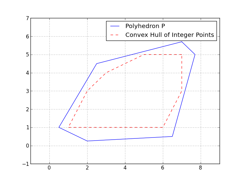
GrUMPy can be used to visualize polyhedra in two dimenions using the module polyhedron (see, e.g., DisplayPolyhedronAndSolveLP.py)

from coinor.grumpy.polyhedron2D import Polyhedron2D, Figure
points = [[2.5, 4.5], [6.5, 0.5], [0.5, 1],
          [7, 5.7], [7.7, 5], [2, 0.25]]
rays = []
c = [2, 5]
opt = [7, 5.7]
loc = (opt[0]+0.1, opt[1]-0.1)
obj_val = 42.5

p = Polyhedron2D(points = points, rays = rays)
f = Figure()
f.add_polyhedron(p, label = 'Polyhedron $P$', color = 'red')
f.set_xlim([p.xlim[0], p.xlim[1]+1])
f.set_ylim([p.ylim[0], p.ylim[1]+2])
f.add_line(c, obj_val, p.xlim + [0.2, 0.8], p.ylim + [0.2, 1.8], 
           linestyle = 'dashed', color = 'black', label = "Objective Function")
f.add_point(opt, 0.04, 'red')
f.add_text(loc, r'$x^* = %s$' % str(opt))
f.show()