Dijkstra's Shortest Path variants for 6, 18, and 26-connected 3D Image Volumes or 4 and 8-connected 2D images.
import dijkstra3d
import numpy as np

field = np.ones((512, 512, 512), dtype=np.int32)
source = (0,0,0)
target = (511, 511, 511)


# If you're working with a binary image with one color considered
# foreground the other background, use this function.
path = dijkstra3d.binary_dijkstra(field, source, target, background_color=0)
path = dijkstra3d.binary_dijkstra(
  field, source, target,
  anisotropy=(2.0, 2.0, 1.0),
)

# path is an [N,3] numpy array i.e. a list of x,y,z coordinates
# terminates early, default is 26 connected
path = dijkstra3d.dijkstra(field, source, target, connectivity=26)
path = dijkstra3d.dijkstra(field, source, target, bidirectional=True) # 2x memory usage, faster

# Use distance from target as a heuristic (A* search)
# Does nothing if bidirectional=True (it's just not implemented)
path = dijkstra3d.dijkstra(field, source, target, compass=True)

# parental_field is a performance optimization on dijkstra for when you
# want to return many target paths from a single source instead of
# a single path to a single target. `parents` is a field of parent voxels
# which can then be rapidly traversed to yield a path from the source.
# The initial run is slower as we cannot stop early when a target is found
# but computing many paths is much faster. The unsigned parental field is
# increased by 1 so we can represent background as zero. So a value means
# voxel+1. Use path_from_parents to compute a path from the source to a target.
parents = dijkstra3d.parental_field(field, source=(0,0,0), connectivity=6) # default is 26 connected
path = dijkstra3d.path_from_parents(parents, target=(511, 511, 511))
print(path.shape)

# Given a boolean label "field" and a source vertex, compute
# the anisotropic euclidean chamfer distance from the source to all labeled vertices.
# Source can be a single point or a list of points. Accepts bool, (u)int8 dtypes.
dist_field = dijkstra3d.euclidean_distance_field(field, source=(0,0,0), anisotropy=(4,4,40))

sources = [ (0,0,0), (10, 40, 232) ]
dist_field = dijkstra3d.euclidean_distance_field(
  field, source=sources, anisotropy=(4,4,40)
)
# You can return a map of source vertices to nearest voxels called
# a feature map.
dist_field, feature_map = dijkstra3d.euclidean_distance_field(
  field, source=sources, return_feature_map=True,
)

# To make the EDF go faster add the free_space_radius parameter. It's only
# safe to use if you know that some distance around the source point
# is unobstructed space. For that region, we use an equation instead
# of dijkstra's algorithm. Hybrid algorithm! free_space_radius is a physical
# distance, meaning you must account for anisotropy in setting it.
dist_field = dijkstra3d.euclidean_distance_field(field, source=(0,0,0), anisotropy=(4,4,40), free_space_radius=300)

# You can also get one of the possibly multiple maxima locations instantly.
dist_field, max_loc = dijkstra3d.euclidean_distance_field(field, source=(0,0,0), return_max_location=True)

# Given a numerical field, for each directed edge from adjacent voxels A and B,
# use B as the edge weight. In this fashion, compute the distance from a source
# point for all finite voxels.
dist_field = dijkstra3d.distance_field(field, source=(0,0,0)) # single source
dist_field = dijkstra3d.distance_field(field, source=[ (0,0,0), (52, 55, 23) ]) # multi-source
dist_field, max_loc = dijkstra3d.distance_field(field, source=(0,0,0), return_max_location=True) # get the location of one of the maxima

# You can also provide a voxel connectivity graph to provide customized
# constraints on the permissible directions of travel. The graph is a
# uint32 image of equal size that contains a bitfield in each voxel
# where each of the first 26-bits describes whether a direction is
# passable. The description of this field can be seen here:
# https://github.com/seung-lab/connected-components-3d/blob/3.2.0/cc3d_graphs.hpp#L73-L92
#
# The motivation for this feature is handling self-touching labels, but there
# are many possible ways of using this.
graph = np.zeros(field.shape, dtype=np.uint32)
graph += 0xffffffff # all directions are permissible
graph[5,5,5] = graph[5,5,5] & 0xfffffffe # sets +x direction as impassable at this voxel
path = dijkstra.dijkstra(..., voxel_graph=graph)
Perform dijkstra's shortest path algorithm on a 3D image grid. Vertices are voxels and edges are the nearest neighbors. For 6 connected images, these are the faces of the voxel (L1: manhattan distance), 18 is faces and edges, 26 is faces, edges, and corners (L∞: chebyshev distance). For given input voxels A and B, the edge weight from A to B is B and from B to A is A. All weights must be finite and non-negative (incl. negative zero).
This package was developed in the course of exploring TEASAR skeletonization of 3D image volumes (now available in Kimimaro). Other commonly available packages implementing Dijkstra used matricies or object graphs as their underlying implementation. In either case, these generic graph packages necessitate explicitly creating the graph's edges and vertices, which turned out to be a significant computational cost compared with the search time. Additionally, some implementations required memory quadratic in the number of vertices (e.g. an NxN matrix for N nodes) which becomes prohibitive for large arrays. In some cases, a compressed sparse matrix representation was used to remain within memory limits.
Neither graph construction nor quadratic memory pressure are necessary for an image analysis application. The edges between voxels (3D pixels) are regular and implicit in the rectangular structure of the image. Additionally, the cost of each edge can be stored a single time instead of 26 times in contiguous uncompressed memory regions for faster performance.
Previous rationals aside, the most recent version of dijkstra3d also includes an optional method for specifying the voxel connectivity graph for each voxel via a bitfield. We found that in order to solve a problem of label self-contacts, we needed to specify impermissible directions of travel for some voxels. This is still a rather compact and fast way to process the graph, so it doesn't really invalidate our previous contention.
#include <vector>
#include "dijkstra3d.hpp"

// 3d array represented as 1d array
float* labels = new float[512*512*512]();

// x + sx * y + sx * sy * z
int source = 0 + 512 * 5 + 512 * 512 * 3; // coordinate <0, 5, 3>
int target = 128 + 512 * 128 + 512 * 512 * 128; // coordinate <128, 128, 128>

vector<unsigned int> path = dijkstra::dijkstra3d<float>(
  labels, /*sx=*/512, /*sy=*/512, /*sz=*/512,
  source, target, /*connectivity=*/26 // 26 is default
);

vector<unsigned int> path = dijkstra::bidirectional_dijkstra3d<float>(
  labels, /*sx=*/512, /*sy=*/512, /*sz=*/512,
  source, target, /*connectivity=*/26 // 26 is default
);

// A* search using a distance to target heuristic
vector<unsigned int> path = dijkstra::compass_guided_dijkstra3d<float>(
  labels, /*sx=*/512, /*sy=*/512, /*sz=*/512,
  source, target, /*connectivity=*/26 // 26 is default
);

uint32_t* parents = dijkstra::parental_field3d<float>(
  labels, /*sx=*/512, /*sy=*/512, /*sz=*/512,
  source, /*connectivity=*/26 // 26 is default
);
vector<unsigned int> path = dijkstra::query_shortest_path(parents, target);


// Really a chamfer distance.
// source can be a size_t (single source) or a std::vector<size_t> (multi-source)
float* field = dijkstra::euclidean_distance_field3d<float>(
  labels,
  /*sx=*/512, /*sy=*/512, /*sz=*/512,
  /*wx=*/4, /*wy=*/4, /*wz=*/40,
  source, /*free_space_radius=*/0 // set to > 0 to switch on
);

// source can be a size_t (single source) or a std::vector<size_t> (multi-source)
float* field = dijkstra::distance_field3d<float>(labels, /*sx=*/512, /*sy=*/512, /*sz=*/512, source);pip install dijkstra3dRequires a C++ compiler.
pip install numpy
pip install dijkstra3dRequires a C++ compiler.
git clone https://github.com/seung-lab/dijkstra3d.git
cd dijkstra3d
virtualenv -p python3 venv
source venv/bin/activate
pip install -r requirements.txt
python setup.py developI ran three algorithms on a field of ones from the bottom left corner to the top right corner of a 512x512x512 int8 image using a 3.7 GHz Intel i7-4920K CPU. Unidirectional search takes about 42 seconds (3.2 MVx/sec) with a maximum memory usage of about 1300 MB. In the unidirectional case, this test forces the algorithm to process nearly all of the volume (dijkstra aborts early when the target is found). In the bidirectional case, the volume is processed in about 11.8 seconds (11.3 MVx/sec) with a peak memory usage of about 2300 MB. The A* version processes the volume in 0.5 seconds (268.4 MVx/sec) with an identical memory profile to unidirectional search. A* works very well in this simple case, but may not be superior in all configurations.
Theoretical unidirectional memory allocation breakdown: 128 MB source image, 512 MB distance field, 512 MB parents field (1152 MB). Theoretical bidirectional memory allocation breakdown: 128 MB source image, 2x 512 distance field, 2x 512 MB parental field (2176 MB).
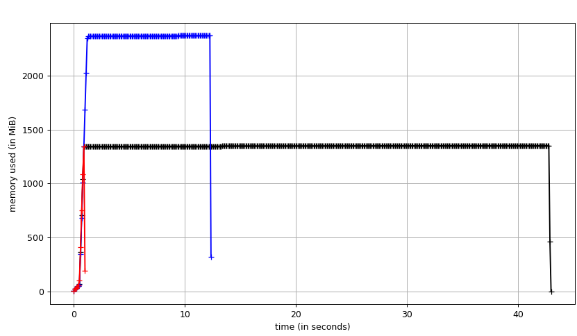
Fig. 1: A benchmark of dijkstra.dijkstra run on a 5123 voxel field of ones from bottom left source to top right target. (black) unidirectional search (blue) bidirectional search (red) A* search aka compass=True.
import numpy as np
import time
import dijkstra3d

field = np.ones((512,512,512), order='F', dtype=np.int8)
source = (0,0,0)
target = (511,511,511)

path = dijkstra3d.dijkstra(field, source, target) # black line
path = dijkstra3d.dijkstra(field, source, target, bidirectional=True) # blue line
path = dijkstra3d.dijkstra(field, source, target, compass=True) # red line
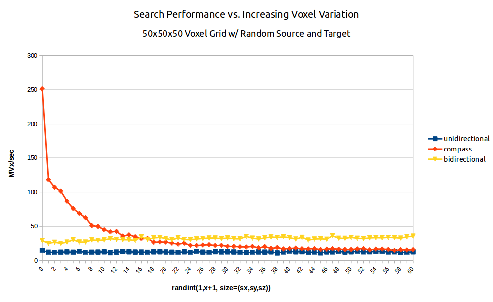
Fig. 2: A benchmark of dijkstra.dijkstra run on a 503 voxel field of random integers of increasing variation from random source to random target. (blue/squares) unidirectional search (yellow/triangles) bidirectional search (red/diamonds) A* search aka compass=True.
import numpy as np
import time
import dijkstra3d

N = 250
sx, sy, sz = 50, 50, 50

def trial(bi, compass):
  for n in range(0, 100, 1):
    accum = 0
    for i in range(N):
      if n > 0:
        values = np.random.randint(1,n+1, size=(sx,sy,sz))
      else:
        values = np.ones((sx,sy,sz))
      values = np.asfortranarray(values)
      start = np.random.randint(0,min(sx,sy,sz), size=(3,))
      target = np.random.randint(0,min(sx,sy,sz), size=(3,))

      s = time.time()
      path_orig = dijkstra3d.dijkstra(values, start, target, bidirectional=bi, compass=compass)
      accum += (time.time() - s)

    MVx_per_sec = N * sx * sy * sz / accum / 1000000
    print(n, ',', '%.3f' % MVx_per_sec)

print("Unidirectional")
trial(False, False)
print("Bidirectional")
trial(True, False)
print("Compass")
trial(False, True)You may optionally provide a unsigned 32-bit integer image that specifies the allowed directions of travel per voxel as a directed graph. Each voxel in the graph contains a bitfield of which only the lower 26 bits are used to specify allowed directions. The top 6 bits have no assigned meaning. It is possible to use smaller width bitfields for 2D images (uint8) or for undirected graphs (uint16), but they are not currently supported. Please open an Issue or Pull Request if you need this functionality.
The specification below shows the meaning assigned to each bit. Bit 32 is the MSB, bit 1 is the LSB. Ones are allowed directions and zeros are disallowed directions.
    32     31     30     29     28     27     26     25     24     23
------ ------ ------ ------ ------ ------ ------ ------ ------ ------
unused unused unused unused unused unused -x-y-z  x-y-z -x+y-z +x+y-z

    22     21     20     19     18     17     16     15     14     13
------ ------ ------ ------ ------ ------ ------ ------ ------ ------
-x-y+z +x-y+z -x+y+z    xyz   -y-z    y-z   -x-z    x-z    -yz     yz

    12     11     10      9      8      7      6      5      4      3
------ ------ ------ ------ ------ ------ ------ ------ ------ ------
   -xz     xz   -x-y    x-y    -xy     xy     -z     +z     -y     +y
     2      1
------ ------
    -x     +x
There is an assistive tool available for producing these graphs from adjacent labels in the cc3d library.
- E. W. Dijkstra. "A Note on Two Problems in Connexion with Graphs" Numerische Mathematik 1. pp. 269-271. (1959)
- E. W. Dijkstra. "Go To Statement Considered Harmful". Communications of the ACM. Vol. 11, No. 3, pp. 147-148. (1968)
- Pohl, Ira. "Bi-directional Search", in Meltzer, Bernard; Michie, Donald (eds.), Machine Intelligence, 6, Edinburgh University Press, pp. 127-140. (1971)

