Fronts is a Python numerical library for nonlinear diffusion problems based on the Boltzmann transformation.

Python 3.9.6 (default, Sep 26 2022, 11:37:49)
>>> import fronts
>>> θ = fronts.solve(D="exp(7*θ)/2", i=0, b=1)  # i: initial value, b: boundary value
>>> θ(r=10, t=3) 
0.9169685387070694
>>> θ.d_dr(10,3)  # ∂θ/∂r
-0.01108790437249313
>>> print("Welcome to the Fronts project page.")

With Fronts, you can effortlessly find solutions to many problems of nonlinear diffusion along a semi-infinite axis r, i.e.:

$$\frac{\partial\theta}{\partial t} = \nabla\cdot\left[D(\theta)\frac{\partial\theta}{\partial r}\mathbf{\hat{r}}\right]$$

where D is a known positive function and θ is an unkown function of r and t.

Fronts includes functionality to solve problems with a Dirichlet boundary condition (start with fronts.solve()), as well as some radial problems with a fixed-flowrate boundary condition (with fronts.solve_flowrate()). In every case, D can be any function defined by the user or obtained from the fronts.D module.

It works by transforming the above nonlinear partial differential equation (PDE) into a more manageable (but still nonlinear) ordinary differential equation (ODE), using a technique known as the Boltzmann transformation, which it then solves with a combination of high-order numerical ODE integration (provided by the SciPy library) and specialized logic.

For this class of problems, you will find that Fronts can be easier to use, faster, and more robust than the classical numerical PDE solvers you would otherwise have to use. Moreover, the solutions found by Fronts are such that their partial derivatives and flux fields are also available in continuous form. Finally, a considerable effort has been made to have Fronts "just work" in practice, with no adjustment of numerical parameters required (in fact, the functions mentioned so far do not even require a starting mesh).

Fronts can also help you solve the inverse problem of finding D when θ is given. Every feature of Fronts is covered in the documentation, and the project includes many example cases (though you may start with the Usage section below).

Fronts is open source and works great with the tools of the SciPy ecosystem.

Problems compatible with Fronts appear in many areas of physics. For instance, if we take θ as the water content or saturation and D as the moisture diffusivity, the above equation translates into what is known as the moisture diffusivity equation, which is a special case of the Richards equation that describes capillary flow in porous media. For this application, Fronts even includes implementations of the commonly used models: fronts.D.brooks_and_corey() and fronts.D.van_genuchten().

Of particular interest to the creators of Fronts is the fact that it can be used to model the configuration known as "lateral flow" in the field of paper-based microfluidics. The name "Fronts" is a reference to the wetting fronts that appear under these conditions, the study of which motivated the creation of this software.

Other problems of this class appear in the study of the diffusion of solutions in polymer matrices as well as diffusion problems in solids (e.g. annealing problems in metallurgy).

As mentioned before, if your problem is supported, you can expect Fronts to be easier to use, faster, and more robust than other tools. Try it out!

Fronts currently runs on Python 3.7 and later.

Install Fronts with pip by running this command in a terminal:

python3 -m pip install fronts

This will download and install the most recent version of Fronts available on PyPI.

Running the bundled examples requires the visualization library Matplotlib. This library is not installed automatically with Fronts, so if you don't already have it, you may want to install it manually by running:

python3 -m pip install matplotlib

Optionally, Fronts can be installed in a virtual environment, or the --user option can be added to the previous commands to install the packages for the current user only (which does not require system administrator privileges).

Let's say we want to solve the following initial-boundary value problem:

Find c such that:

$$ \begin{cases} \dfrac{\partial c}{\partial t} = \dfrac{\partial}{\partial r}\left(c^4\dfrac{\partial c}{\partial r}\right) & r>0,t>0\\ c(r,0)=0.1 & r>0\\ c(0,t)=1 & t>0\\ \end{cases} $$

With Fronts, all it takes is a call to fronts.solve(). The function requires the diffusivity function D, which we pass as an expression so that solve() can get the derivatives it needs by itself (alternatively, in this case we could also have used fronts.D.power_law() to obtain D). Besides D, we only need to pass the initial and boundary values as i and b. The Python code is:

import fronts
c = fronts.solve(D="c**4", i=0.1, b=1)

The call to solve() finishes within a fraction of a second. c is assigned a Solution object, which can be called directly but also has some interesting methods such as d_dr(), d_dt() and flux().

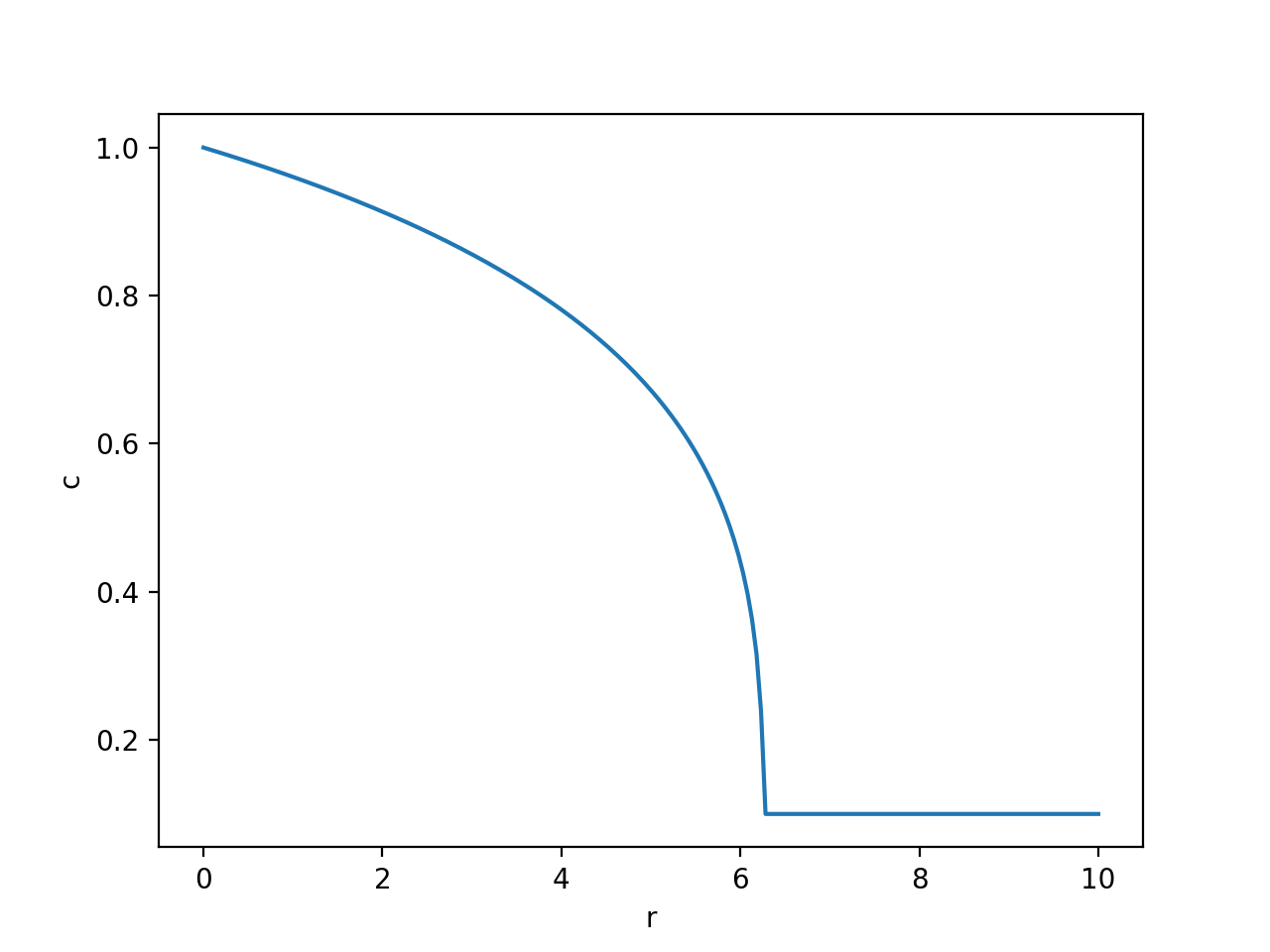
We can now plot the solution for arbitrary r and t. For example, with r between 0 and 10 and t=60:

import numpy as np
import matplotlib.pyplot as plt

r = np.linspace(0, 10, 200)
plt.plot(r, c(r, t=60))
plt.xlabel("r")
plt.ylabel("c")
plt.show()

The plot looks like this:

Finally, let us plot the flux at t=60:

plt.plot(r, c.flux(r, t=60))
plt.xlabel("r")
plt.ylabel("flux")
plt.show()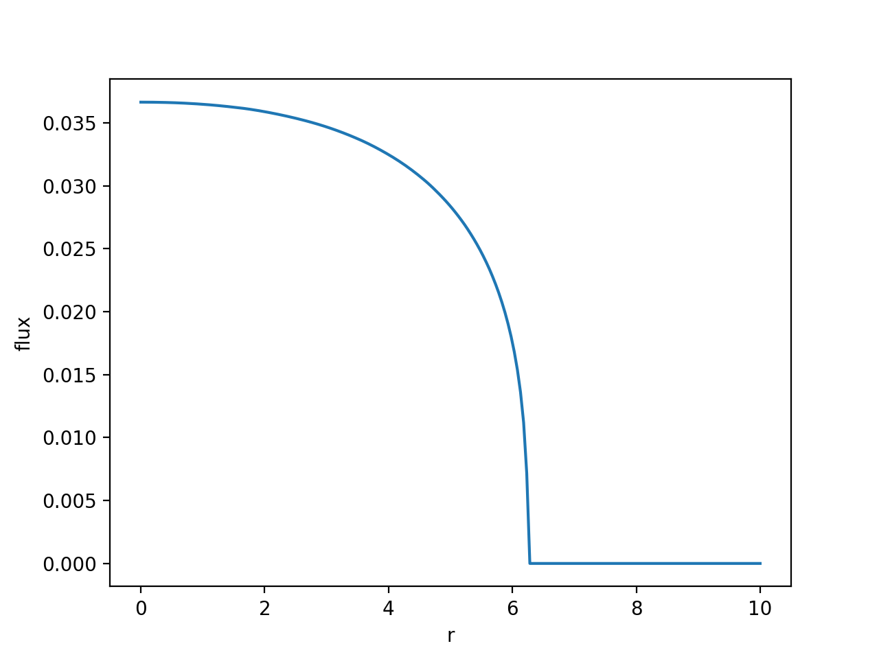

• Documentation
• Examples
• Changelog
• Capillarity paper

• Gabriel S. Gerlero @gerlero
• Pablo A. Kler @pabloakler
• Claudio L. A. Berli

Fronts was conceived and is developed by members of the Santa Fe Microfluidics Group (GSaM) at the Research Center for Computational Methods (CIMEC, UNL-CONICET) and the Institute of Technological Development for the Chemical Industry (INTEC, UNL-CONICET) in Santa Fe, Argentina.

Fronts is open-source software available under the BSD 3-clause license.