LDR stands for Latent Dimensionality Reduction. It is a generic method for interpreting models and making accurate predictions when features are missing. It is deployed here as a python module.

About

The purpose of LDR is to solve a common data science problem. Often models that have a higher predictive accuracy are more complex. These complex models are sensibly referred to as black box models. This is frustrating for many data scientists, as they end up with a model that performs well, but can't explain why. Inability to explain the model frequently causes the model to fail in critical situations, that are difficult to test for. Also, black box models typically require all features to be present to make a prediction. LDR provides a solution to both of these problems.

Getting Started

Prerequesites

Python3.

Note: Some examples contain additional that are not installed as dependencies by default, such as PyTorch.

Installation

python3 -m pip install ldr --user

Examples

An example analysis of a classification problem can be found here.

Imputation from density

After calculating the density estimate of the trained model using density_estimate(), using predict() on new data will automatically impute missing features.

Note: currently only missing columns will be imputed, not the odd value here or there.

Note: This has not been fully implemented, so the optimal accuracy has not been achieved, and it's a bit slow. Contribution welcome :).

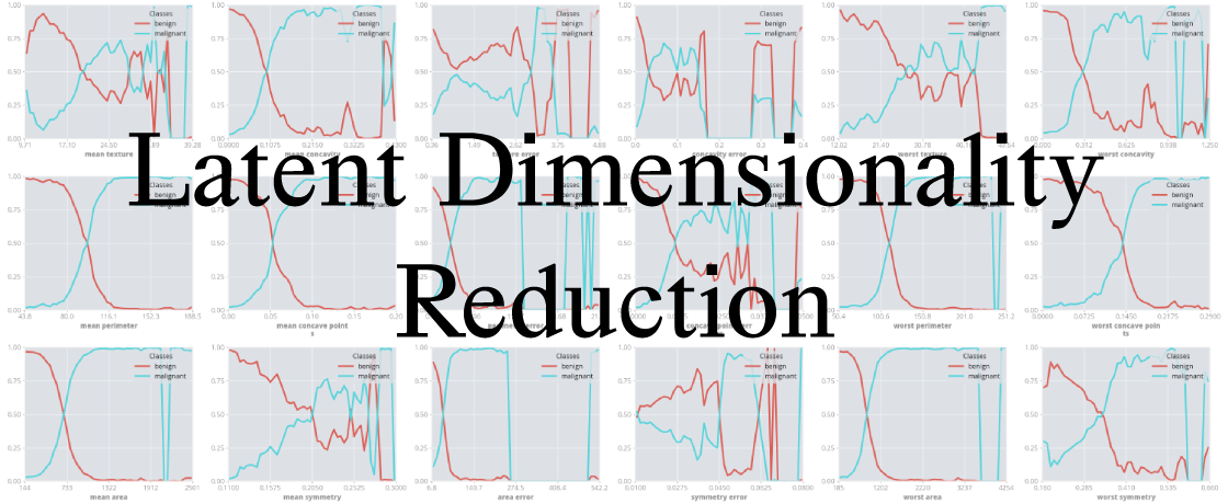
Visualizations

The examples above generate either 1D or 2D visualizations. These demonstrate the certainty of the model across the sample space it is trained on. Take the 1D visualizations from the classification example, which describe the model's certainty of malignancy classification of mean area and area error of breast cancer samples in a study.

1 Dimensional Visualization

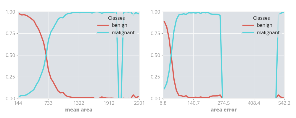
Here what can be seen is that if a cancer has a mean area of less than 250 then the model is most likely to classify it as benign, whereas if it has a mean area of more than 1200 then it is almost certainly going to be classified as malignant.

With the area error, what can be seen is that between 280 and 480, there is not enough training data for the model to reliably make a prediction in that area, as the total model certainty drops to 0 for both classifications. Between 80 and 210 the model is very biased towards a malignant classification.

2 Dimensional Visualization

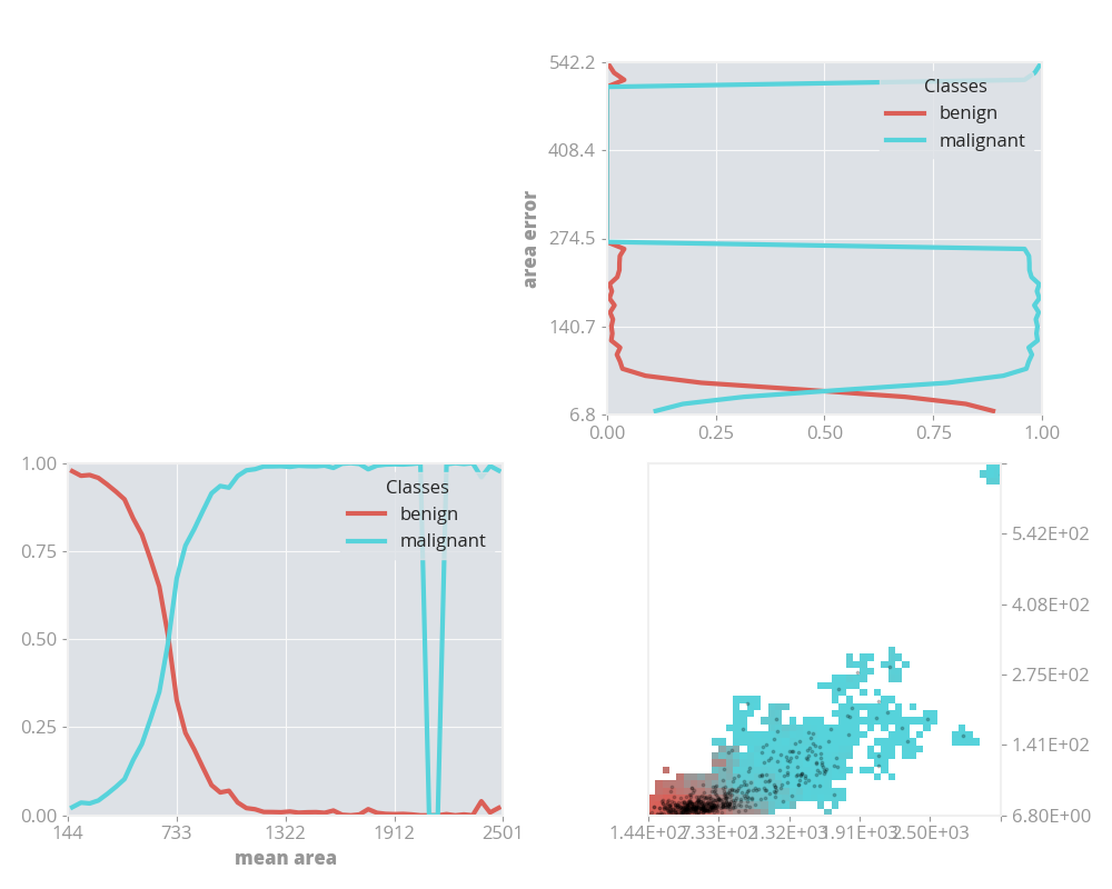
Interpolating two classification certainties of individual features results in the heatmap in the bottom right. What can be seen is that the majority of samples have a low mean area and a low area error. When samples deviate away from the bottom left, with increasing mean area and area errors, the probability of a malignancy classification dramatically increases.

n Dimensional Visualizations

Even though only 1 and 2 dimensional visualizations are given, the entire classifier certainty across the sample space has been mapped. In this study there are actualy 30 features, but by using LDR the individual components can be easily extracted. In order for a human to interpret an algorithmic model, they must be able to see it. As Donald Knuth says:

"An algorithm must be seen to be believed, and the best way to learn what an algorithm is all about is to try it."

Note: most successful black box models come from algorithmic techniques, such as neural networks; this is why I draw this similarity.

Why LDR is Better Than Naive Techniques

Naive techniques for analysis black box models consist of analysing individual features (or composite functions of features) directly against their classifications resulting from each sample in the sample space. Because of this, the extrapolation that happens when applying the model to real world situations is never experimented against. Because LDR draws samples randomly from a KDE (kernel density estimate) of the sample space, by default there is extrapolation. Because of the KDE of the model, features can be imputed during prediction by taking the typical value of variables at the highest density, giving a more accurate representation of the feature space.

The LDR Recipe

As machine learning algorithms go, LDR is pretty simple. It's effectively just a monte-carlo integration across the sample space, using the VEGAS algorithm as the sampling method.

1. Min-max scale the data so that it falls into [0, 1] intervals.

2. Train a predictive model on the scaled data.

3. Create a kernel density estimate of the training samples.

4. Sample n new points from the kernel density estimate, using the predictive model to make a prediction at each point.

5. Bin the samples according to regular intervals. For each dimension, group points with resolution r, reducing the value of the bin to the mean prediction across it.

See the paper for more detail.

Additional Notes

If you find this package useful, please consider contributing!