LogicalLens

A "logical lens" is a map: f : Data -> ([0, 1]^n -> bool) and is interpreted as a family of properties over the hyper unit box, [0, 1]^n, indexed by "Data". Further, f(data) must be monotonic threshold function. That is, given a fixed data data, the map g = f(data) is such that for any two points in the unit box, x, y in [0, 1]^n if x <= y coordinate-wise, then g(x) <= g(y) , where False <= True. An example is given below (see monotone-bipartition for details):

In principle, Data can be anything from time-series to pictures of dogs. The key idea is that a logical lens enables leveraging domain specific knowledge in the form of property tests to design features and similarity measures.

For details on this formalism, see the following two papers or this slide deck:

1. Vazquez-Chanlatte, Marcell, et al."Time Series Learning using Monotonic Logical Properties.", International Conference on Runtime Verification, RV, 2018

2. Vazquez-Chanlatte, Marcell, et al. "Logical Clustering and Learning for Time-Series Data." International Conference on Computer Aided Verification. Springer, Cham, 2017.

Usage

Example Dataset

We begin by defining a dataset. Here we focus on some toy "car speeds" with the goal of detecting traffic "slow downs" (see below). While a bit contrived, this example will illustrate the common workflow of this library.

This dataset is provided in example_data/toy_car_speeds. Below, we assume that data is a list of the 6 piece-wise constant time series, where each element is a sequence of (timestamp, value) pairs. For example,

print(data[5])  # [(0, 0.1)]

Code for loading the data is given in example/toy_car_speeds/load.py.

Example Specification

We can now define a monotonic parametric properties we are interested in testing. To continue our example, let us test if the car's speed remains below some value h after time tau.

def slow_down_lens(data):
    def spec(params):
        h, tau = params
        tau *= 20
        return all(speed < h for t, speed in data if t >= tau)
    return spec

Since we require each parameter to be between 0 and 1, we rescale tau to be between 0 and 20 internally. Further, because the car's speed is already normalized between 0 and 1, h does not need to change.

Finally, before moving on, notice that slow_down_lens is indeed monotonic since increasing h and tau both make the property easier to satisfy.

Aside

For more complicated specifications using temporal logic, we recommend using the metric-temporal-logic library.

Example Usage

We are finally ready to use the logical_lens library. We begin by bringing the LogicalLens class into scope. This class wraps a mathematical logical lens into an easy to use object.

from logical_lens import LogicalLens

lens = LogicalLens(n=2, lens=slow_down_lens)

Under this lens, the time series become threshold surfaces in the 2-d unit box (see fig below). If needed, these threshold boundaries can be approximated as a series of rectangles. Example code to compute the rectangles is given below.

recs = lens.boundary(data[5], approx=True, tol=1e-4)  # List of rectangles

In practice, one typically need not work with the threshold boundaries directly. For example, one may wish to compute the induced "Logical Distance" (hausdorff distance of boundaries) between data.

# Compute Logical Distances.
d = lens.dist(data[0], data[1])
A = lens.adj_matrix(data=data)  # Compute full adjacency matrix.

As pointed out in the reference papers, the logical distance is in general quite slow to compute. Often, it is advantageous to use a coarse characterization and then refine this characterization as needed. For example, consider computing the unique intersection of a line from the origin and the threshold surfaces. If two boundaries are close together, then they need to have similar intersection points. We show below how to do this using logical_lens. Note that instead of the intersection point, we return how far along the line [0, 1] the intersection occurs.

points = [
    (0, 1),   # Reference line intersecting origin and (0, 1)
    (1, 0.3)  # ..                                     (1, 0.3)
]
f = lens.projector(points)  # Note, will project to -1 or 2 if no intersection
                            # is found.
Y = [f(d) for d in data]

Because one cannot know where to project a-priori, we support generating a projector on n random lines.

## Project onto 2 random lines.
f2 = lens.random_projector(2)

We also support finding the point on the threshold boundaries according to some lexicographic ordering (see Vazquez-Chanlatte, el al, CAV 2017).

## Project using lexicographic ordering of parameters:
f3 = lens.lex_projector(orders=[
   [(1, False), (0, True)],  # minimizing on axis 1 then maximizing on axis 0.
   [(0, False), (1, False)],  # minimizing on axis 0 then minimizing on axis 1.
])

Using with Scikit learn

Finally, we give an example of how to use this tool with scikit learn.

import numpy as np
from sklearn.mixture import GaussianMixture

Suppose we have much more time-series:

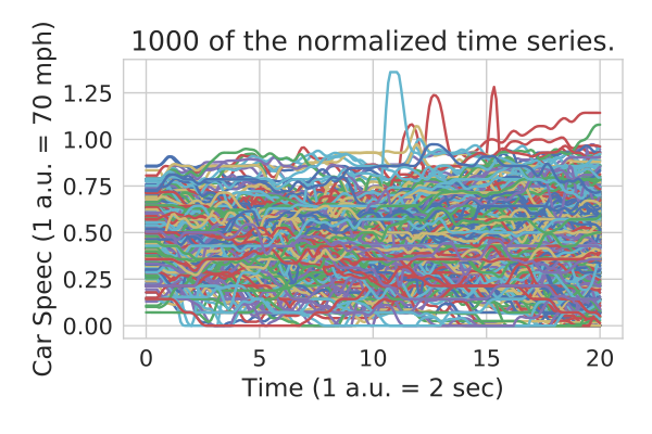
We start by computing a coarse classification of the time series by projecting onto two random lines and then learning a Gaussian Mixture Model to find clusters.

# Project data down to two dimensinos.
f = lens.projector([(0.5, 1), (1, 0.2)])
X = np.vstack([f(d) for d in data])  # collect projected data into a matrix.

# Throw out data that had no intersections (and thus no slow downs).
intersects = (data != 2).T[0] * (data != 2).T[1]
X = X[intersects]

# Learn a guassian mixture model
model = GaussianMixture(5)
model.fit(X)

labels = np.array([model.predict(x.reshape(1,2))[0] for x in X])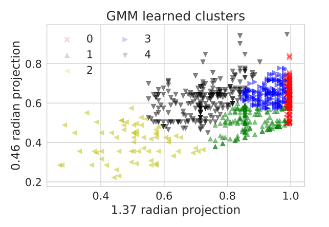

By checking which cluster the 0 toy time series belongs to, we identify cluster 4 as potential slow down. We can then compute the logical distance of each datum in cluster 4 to the toy data.

ref = .. # toy_data[0]

dists = [lens.dist(ref, d) for d in data]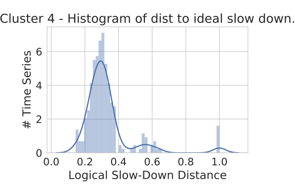

We can see that the distances cluster near 0.35. Annotating the cluster with how far from the toy data gives a classifer "slow down" as the data less than 0.45 distance away from the reference slowdown under our logical lens in cluster 4.

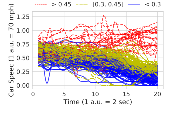
To extract a specification for the learned cluster, one can use the technique described in (Vazquez-Chanlatte et al, CAV 2017). We begin by seeing the range of parameters the slow downs take.

slow_downs = ..  # data identified as slow downs

f1 = lens.projector([(0.5, 1)], percent=False)
f2 = lens.projector([(1, 0.2)], percent=False)
X1 = np.vstack([f1(d) for d in slow_downs])
X2 = np.vstack([f2(d) for d in slow_downs])

box1 = X1.min(axis=0), X1.max(axis=0)  # (0.25, 0.55), (0.38, 0.76)
box2 = X2.min(axis=0), X2.max(axis=0)  # (0.35, 0.17), (0.62, 0.31)

Each box above is implicilty defined a tuple of the point closest to the origin and the on farthest from the origin. The corresponding specification, (given here in Signal Temporal Logic) is: