pyScatSpheres
Package for solving the scalar wave equation with a linear array of scattering spheres. Possibility to solve for constant potential well and hard spheres i.e. infinite potential.
Installation
pip install pyScatSpheres
The installation requires external system based installations :
- Fortran compiler : to run external library py3nj
- optional tex compiler : necessary for the figures to be displayed in latex text.
Those packages can be installed on linux with
apt-get install gfortranapt-get install tex-live
Using the GUI
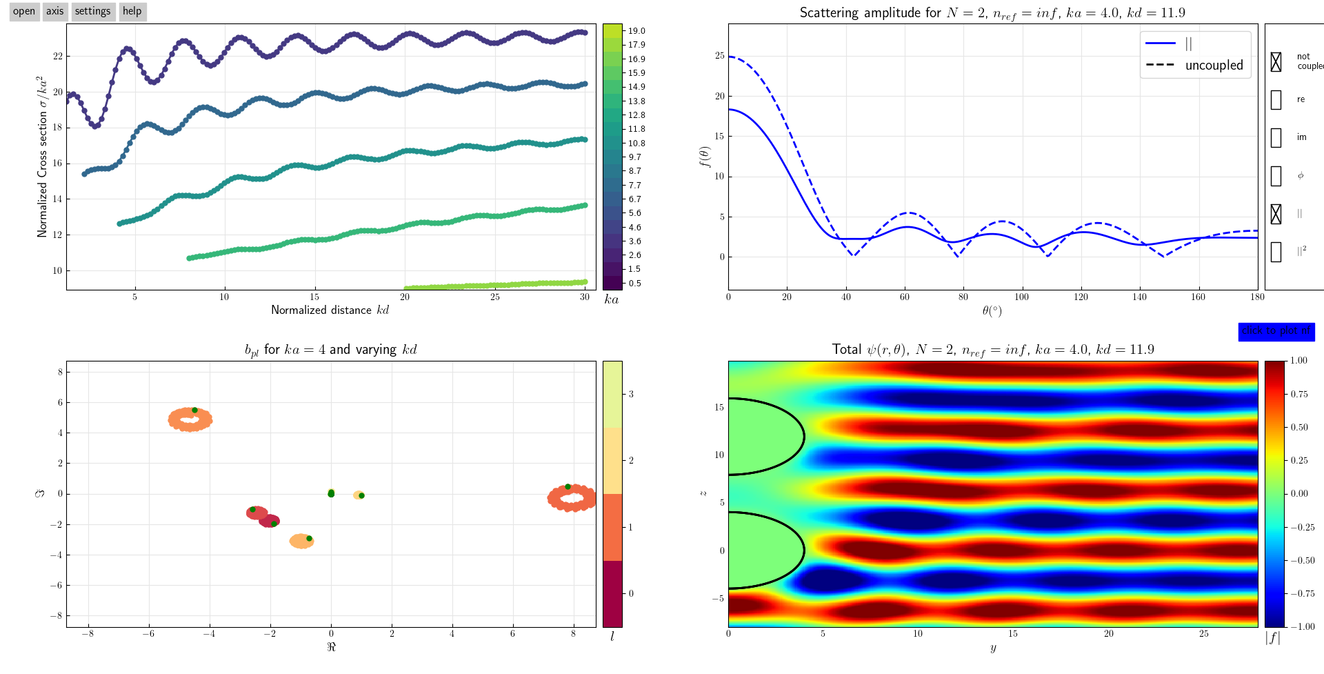
A gui is available to interactively display pre calculated solutions.
import os
from pyScatSpheres import gui_base as hsa_gui

#fetch built-in solution
df_path=os.path.dirname(hsa_gui.__file__)+'/data/qdotSphereArray2_kp0.pkl'
hsa_e = hsa_gui.GUI_handler(df_path)
Using the API
New sets of solution can be calculated and solved to a pickle using the API.
import numpy as np
import pandas as pd
from pyScatSpheres import qdot_sphere_array as qsa
from pyScatSpheres import glob_colors as colors

kas = [0.5,2,5]
kds = [2,5,10]
kps = [1.2]
kas,kps,kds = np.meshgrid(kas,kps,kds)
kas,kps,kds = kas.flatten(),kps.flatten(),kds.flatten()
cols = ['N','ka','kp','kd','nmax','sigma','ap','bp']
df = pd.DataFrame(columns=cols)
for ka,kp,kd in zip(kas,kps,kds):
    nmax = max(int(np.ceil(1.3*ka)),int(ka)+4)
    s = qsa.QdotSphereArray(N=N,ka=ka,kp=kp,kd=kd*ka,nmax=10,solve=1,copt=1)
    sig = s.get_s(npts=1000)
    df=df.append(dict(zip(cols,[s.N,s.ka,s.kp,s.kd,s.nmax,sig,s.ap,s.bp])),ignore_index=True)
df.to_pickle(df_name)
print(colors.green+'DataFrame saved:\n'+ colors.yellow+df_name+colors.black)