PyPólyaGamma

This is a Cython port of Jesse Windle's code at https://github.com/jwindle/BayesLogit. It provides a Python interface for efficiently sampling Pólya-gamma random variates. Install with:

pip install pypolyagamma

Please open issues if you have any trouble!

Background

Pólya-gamma augmentation is a method of performing fast and simple Bayesian inference in models with Gaussian latent variables and count observations. While such models are non-conjugate, if it has the right form (specifically, if it is a Bernoulli, binomial, negative binomial, or multinomial with a logistic link function), we can introduce a set of Pólya-gamma auxiliary variables that render it conditionally conjugate. This facilitates fast Gibbs sampling algorithms on an extended space of Gaussian latent variables and Pólya-gamma auxiliary variables, where integrating out the auxiliary variables leaves the original model intact.

Given the auxiliary variables, the latent Gaussian variables have a Gaussian conditional distribution. Likewise, given the Gaussian latent variables and the observed count data, the auxiliary variables have a Pólya-gamma conditional distribution. Thus, to implement the Gibbs sampling algorithm, we must be able to efficiently sample Pólya-gamma random variates. This library provides code to do exactly that.

The augmented density, the non-Gaussian marginal, and the Gaussian conditionals are illustrated in the figure below. In this case, the posterior is from a simple binomial model. Next, we'll show how to perform Gibbs sampling for such a model.

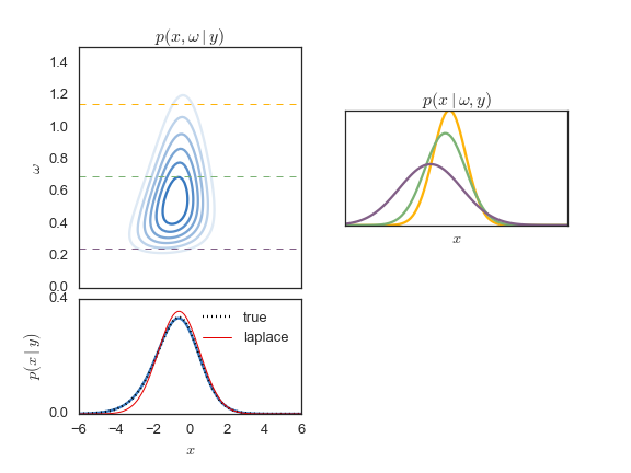
See below for more references and links.

Demo

For convenience, we have created classes for simple count regression models, like the Bernoulli, binomial, negative binomial, and multinomial (with stick breaking) observation models. For example, you can fit a Bernoulli regression as follows:

from pypolyagamma import BernoulliRegression
D_out = 1     # Output dimension
D_in = 2      # Input dimension
reg = BernoulliRegression(D_out, D_in)

# Given X, an NxD_in array of real-valued inputs,
# and Y, and NxD_out array of binary observations. Fit
# the linear model y_n ~ Bern(sigma(A x_n + b)),
# where sigma is the logistic function.  A is D_out x D_in,
# b is D_out x 1, and the entries in y_n are cond. indep.
samples = []
for _ in range(100):
   reg.resample((X,Y))
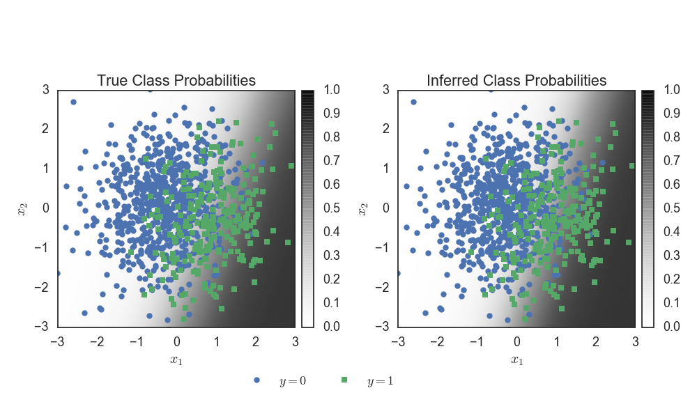
   samples.append((reg.A, reg.b))

Under the hood, this will instantiate Pólya-gamma auxiliary variables and perform conditionally-conjugate Gibbs sampling. We can visualize the inferred parameters in terms of the implied probability for each point in the input space.

Here's how you can manually perform inference in a simple binomial model with N=10 counts and probability p=logistic(x), with a standard normal prior on x.

First, sample a count from the model:

from pypolyagamma import logistic, PyPolyaGamma

# Consider a simple binomial model with unknown probability
# Model the probability as the logistic of a scalar Gaussian.
N = 10
mu = 0.0
sigmasq = 1.0
x_true = npr.normal(mu, np.sqrt(sigmasq))
p_true = logistic(x_true)
y = npr.binomial(N, p_true)

Now we can run a Gibbs sampler to estimate the posterior distribution of x given y.

# Gibbs sample the posterior distribution p(x | y)
# Introduce PG(N,0) auxiliary variables to render
# the model conjugate.  First, initialize the PG
# sampler and the model parameters.
N_samples = 10000
pg = PyPolyaGamma(seed=0)
xs = np.zeros(N_samples)
omegas = np.ones(N_samples)

# Now run the Gibbs sampler
for i in range(1, N_samples):
    # Sample omega given x, y from its PG conditional
    omegas[i] = pg.pgdraw(N, xs[i-1])

    # Sample x given omega, y from its Gaussian conditional
    sigmasq_hat = 1./(1. / sigmasq + omegas[i])
    mu_hat = sigmasq_hat * (mu / sigmasq + (y - N / 2.))
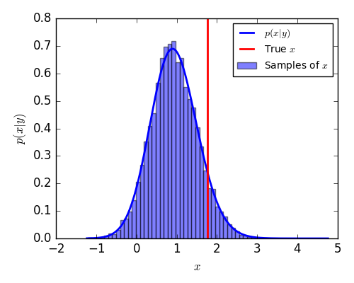
    xs[i] = npr.normal(mu_hat, np.sqrt(sigmasq_hat))

For this simple example, we can compute the true posterior and compare the samples to the target density.

Manual Installation

You can also install from source, but you'll need cython.

pip install cython    
git clone git@github.com:slinderman/pypolyagamma.git
cd pypolyagamma
pip install -e .

To check if it worked, run:

pip install nose
nosetests

If all the tests pass then you're good to go!

Under the hood, the installer will download GSL, untar it, and place it in deps/gsl. It will then configure GSL and compile the Pólya-gamma code along with the required GSL source files. This way, you don't need GSL to be installed and available on your library path.

Parallel sampling with OpenMP

By default, the simple installation above will not support parallel sampling. If you are compiling with GNU gcc and g++, you can enable OpenMP support with the flag:

USE_OPENMP=True pip install -e .

Mac users: you can install gcc and g++ with Homebrew. Just make sure that they are your default compilers, e.g. by setting the environment variables CC and CXX to point to the GNU versions of gcc and g++, respectively. With Homebrew, these versions will be in /usr/local/bin by default.

To sample in parallel, call the pgdrawvpar method:

n = 10             # Number of variates to sample
b = np.ones(n)     # Vector of shape parameters
c = np.zeros(n)    # Vector of tilting parameters
out = np.empty(n)  # Outputs

# Construct a set of PolyaGamma objects for sampling
nthreads = 8
seeds = np.random.randint(2**16, size=nthreads)
ppgs = [pypolyagamma.PyPolyaGamma(seed) for seed in seeds]

# Sample in parallel
pypolyagamma.pgdrawvpar(ppgs, b, c, out)