MINT - Mimetic INTerpolation on the Sphere

Overview

This project provides interpolating and regridding capability to horizontal edge/face centred fields on the sphere.

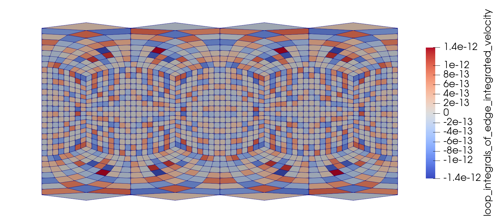
MINT conserves lateral fluxes or vorticity, depending on the field's staggering. The regridding method is mimetic in the sense that Stokes's or the divergence theorems are satisfied to near machine precision. In particular, the loop integrals of an interpolated vector field deriving from a gradient or streamfunction is zero.

The source and destination grids are stored as a collection of grid cells with four vertices each (i.e. the cells are quadrilaterals). MINT can read data stored in a 2D subset version of the UGRID format.

Thank you

The development of the numerical method and its implementation are supported by the Next Generation Modelling Systems effort at the UK Met Office, the National Institute for Water and Atmospheric (NIWA) research and the New Zealand eScience Infrastructure (NeSI).

References

Please refer to the following publications when using MINT.

• MINT: a library that conserves vorticity or lateral fluxes when interpolating vector fields
• Mimetic Interpolation of Vector Fields on Arakawa C/D Grids.
• Conservative interpolation of edge and face data on n dimensional structured grids using differential forms.

Want to contribute?

We're looking for contributions, particularly in the areas of:

• code documentation
• identifying scientific applications that can leverage MINT

Any help will be greatly appreciated.

How to install or build MINT as a Python module

This lets you evaluate MINT with minimal fuss. Note: not all the functionality from C++ is exposed in the Python module -- additional features can be added on request.

We recommend you install Miniconda3. Miniconda installers can be downloaded for Windows, Linux and Mac OS X (here)[https://docs.conda.io/en/latest/miniconda.html].

Conda installation

Once Miniconda3 is installed, type

conda install -c conda-forge python-mint

Note that you will need to have OpenGL, a core dependency of VTK, installed. On Ubuntu, you might have to apt-get install libgl1-mesa-glx.

Building from source

This requires a recent C++ compiler (Visual C++ 2019, gcc 10, clang 12 or later).

conda env create --file requirements/mint.yml
conda activate mint-dev

If you find the above commands to fail on Windows, try (in the Anaconda prompt terminal):

conda create -n mint-dev python=3.9
conda activate mint-dev
conda install -c conda-forge cmake cython setuptools tbb-devel pip libnetcdf vtk numpy pytest netcdf4

Then type:

pip install --no-deps --editable .

Testing the Python module

Check that you can import the mint module:

python -c "import mint"

To run the tests type:

pytest

in the top MINT diretory.

Python module documentation

pydoc mint
pydoc mint.regrid_edges
pydoc mint.polyline_integral

for instance.

Python jupyter notebooks

Below are examples showing how to use MINT from Python.

Interpolating a vector field from cubed-sphere to uniform lon-lat

How to build the MINT C++ Library

If you want to call MINT from Fortran, C or C++ we recommend that you build the mint library. In addition to the C++ and, optionally, the Fortran compilers you will need

• CMake
• NetCDF (libnetcdf) and optionally Fortran NetCDF (libnetcdff)
• VTK >= 9

installed.

In the top MINT directory:

mkdir build
cd build
cmake ..
make -j 8

You can specify the compiler, for instance:

FC=pgfortran CXX=pgcxx cmake ..
make -j 8

The locations of the NetCDF library and headers can be inferred from the nc-config. Use

cmake -D BUILD_FORTRAN=ON ..

to build the Fortran interface (requires libnetcdff to be installed).

You can also specify the location of VTK and NetCDF manually. For instance, in the Anaconda prompt terminal on Windows 10 Entreprise:

call "C:\Program Files (x86)\Microsoft Visual Studio\2019\Community\VC\Auxiliary\Build\vcvars64.bat"
cmake -G "NMake Makefiles" -DVTK_INCLUDE_DIR="%userprofile%\miniconda3\envs\mint-dev\Library\include\vtk-9.0" -DVTK_LIBRARY_DIR="%userprofile%\miniconda3\envs\mint-dev\Library\lib" -DNETCDF_INCLUDE_DIRS="%userprofile%\miniconda3\envs\mint-dev\Library\include" -DNETCDF_LIBRARIES="%userprofile%\miniconda3\envs\mint-dev\Library\lib\netcdf.lib" ..
nmake

Check that the build was successful by typing:

ctest

C++ and Fortran API documentation

https://pletzer.github.io/mint/html/

Examples and applications

Computing flux integrals across irregular boundaries

The two plots below show monthly averaged ocean data computed with the NEMO code (courtesy of Erik Behrens, NIWA). The u and v velocities are staggered according to Arakawa C. From these components, vertically integrated fluxes are assigned to each horizontal cell face. The absolute value of the cell flux intensities are shown on a grey scale on the cell edges.

Open and closed target lines are shown as blue, representing vertically extruded surfaces. The total flux (water flow) is displayed at the bottom left of each picture in millions of cubic metres per second. The direction of the flow is indicated by the arrows. Note that the target lines can interesect land without the need for any form of masking - land has simply the property of zero flux (beige edges).

Gulf Stream:

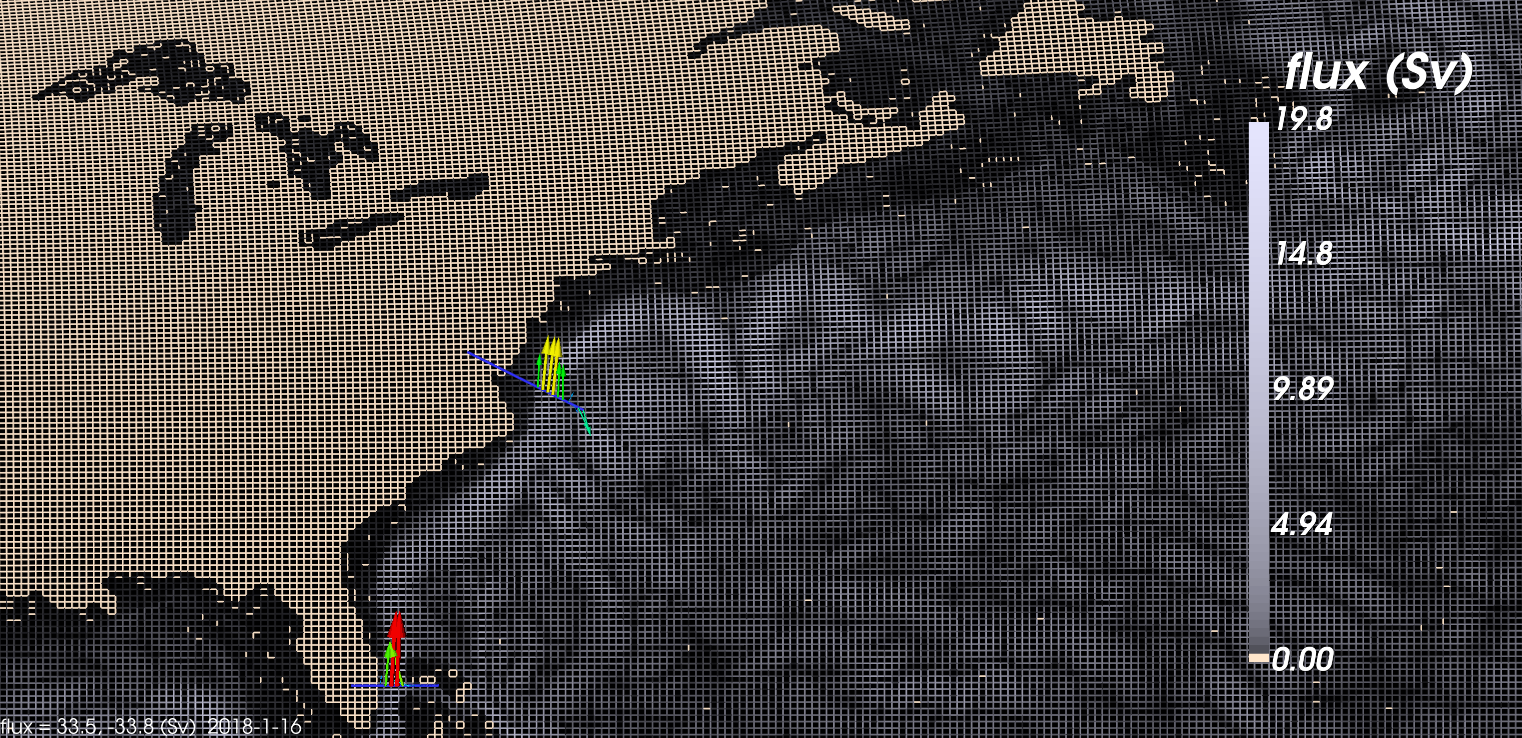
Around New Zealand:

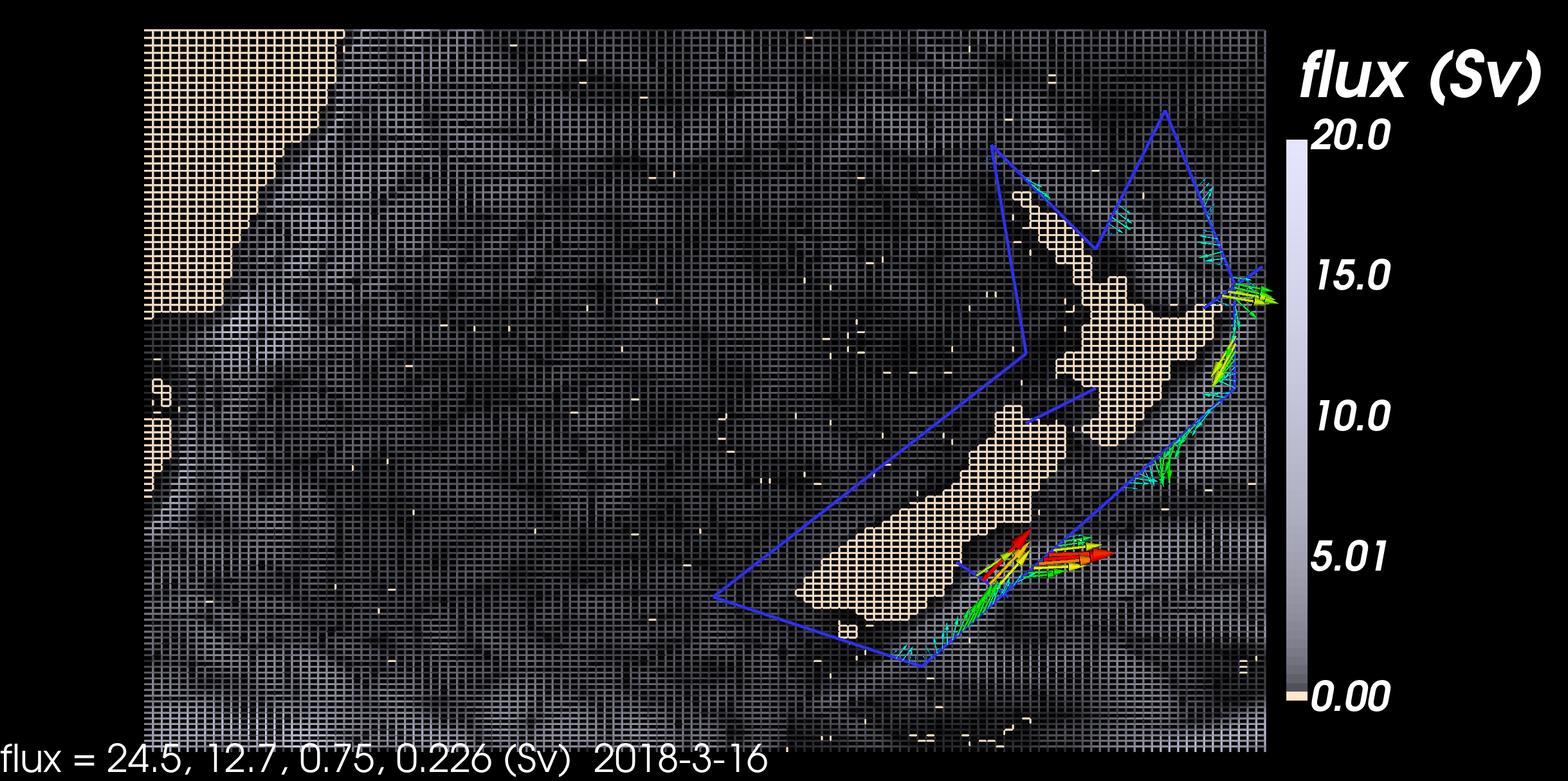
The "tartan" graphics were generated by the fluxviz script in the nemoflux repo.

Advection of a vector field

How do you transport a vector field in a conservative way? The Lie operator governs the evolution of differential forms (nodal, edge, face and cell discretised fields). The integral of the form over its supporting element is invariant in time. For vertical fluxes or 1-forms, the line integrals of the field don't change as the field is carried by the vector field.

This movie shows the edges of a cubed-sphere grid, which are colour coded according the intensity of the fluxes on the edges. Initially, the field is zero everywhere except over a small rectangular region in longitude-latitude space. The advecting vector field is shown as an arrow plot. Over time the field gets transported, spreading and spiralling. MINT was used to set the new field field values by interpolating the field at the previous time step on the edge geometry at the previous time step.

Conservation Error

The plot below shows the error of mimetic regridding error obtained by computing the closed line integral for each cell on the cubed-sphere, which have highly distorted cells near the poles in longitude-latitude coordinates.