![]()
A toolkit to evaluate neural network explanations
PyTorch and TensorFlow
![]()
![]()

Quantus is currently under active development so carefully note the Quantus release version to ensure reproducibility of your work.
News and Highlights! 🚀
- New metrics added: EfficientMPRT and SmoothMPRT by Hedström et al., (2023)
- Released a new version here
- Accepted to Journal of Machine Learning Research (MLOSS), read the paper
- Offers more than 30+ metrics in 6 categories for XAI evaluation
- Supports different data types (image, time-series, tabular, NLP next up!) and models (PyTorch, TensorFlow)
- Extended built-in support for explanation methods (captum, tf-explain and zennit)
Citation
If you find this toolkit or its companion paper Quantus: An Explainable AI Toolkit for Responsible Evaluation of Neural Network Explanations and Beyond interesting or useful in your research, use the following Bibtex annotation to cite us:
@article{hedstrom2023quantus,
  author  = {Anna Hedstr{\"{o}}m and Leander Weber and Daniel Krakowczyk and Dilyara Bareeva and Franz Motzkus and Wojciech Samek and Sebastian Lapuschkin and Marina Marina M.{-}C. H{\"{o}}hne},
  title   = {Quantus: An Explainable AI Toolkit for Responsible Evaluation of Neural Network Explanations and Beyond},
  journal = {Journal of Machine Learning Research},
  year    = {2023},
  volume  = {24},
  number  = {34},
  pages   = {1--11},
  url     = {http://jmlr.org/papers/v24/22-0142.html}
}
When applying the individual metrics of Quantus, please make sure to also properly cite the work of the original authors (as linked below).
Table of contents
Library overview
A simple visual comparison of eXplainable Artificial Intelligence (XAI) methods is often not sufficient to decide which explanation method works best as shown exemplarily in Figure a) for four gradient-based methods — Saliency (Mørch et al., 1995; Baehrens et al., 2010), Integrated Gradients (Sundararajan et al., 2017), GradientShap (Lundberg and Lee, 2017) or FusionGrad (Bykov et al., 2021), yet it is a common practice for evaluation XAI methods in absence of ground truth data. Therefore, we developed Quantus, an easy-to-use yet comprehensive toolbox for quantitative evaluation of explanations — including 30+ different metrics.
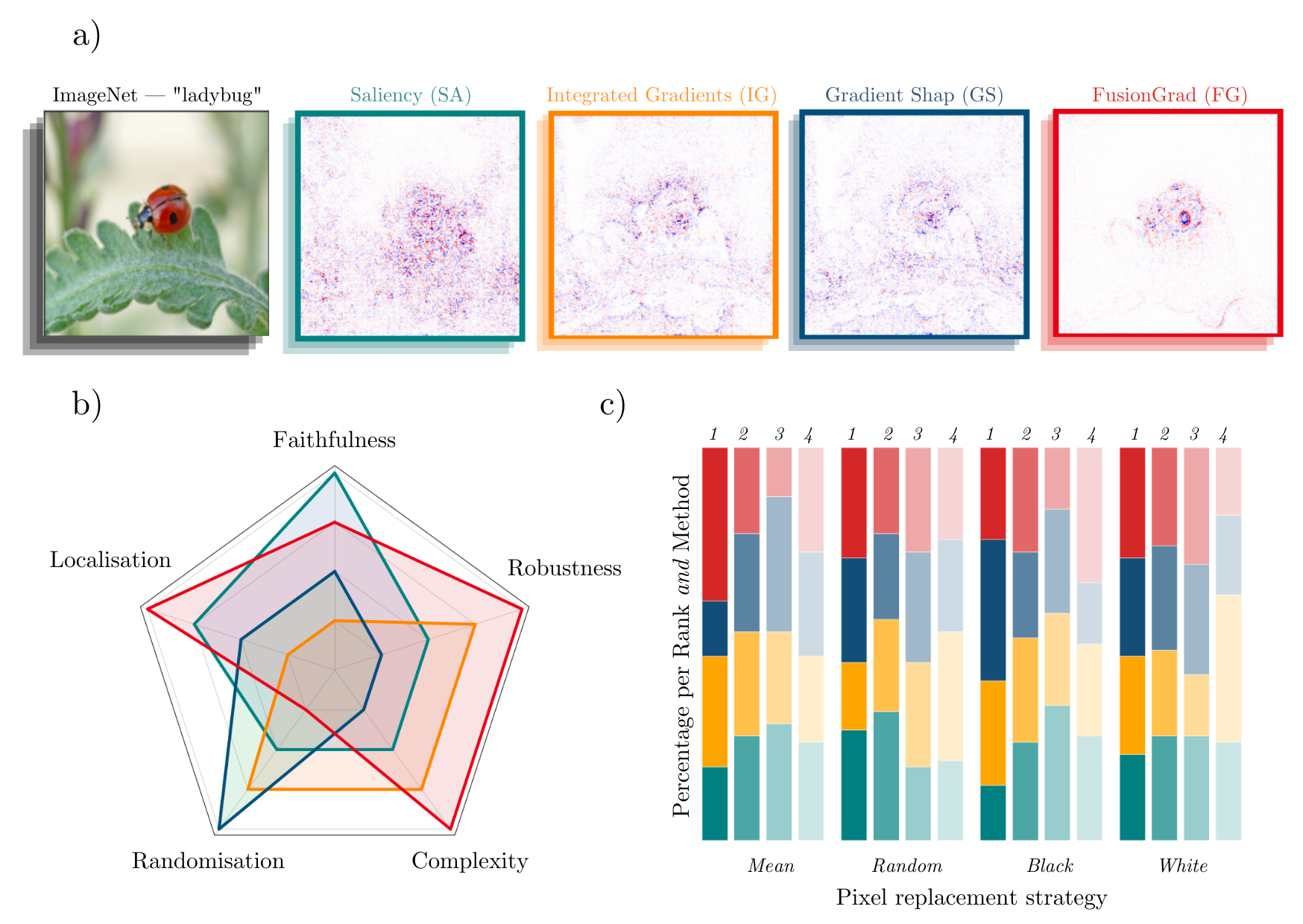
With Quantus, we can obtain richer insights on how the methods compare e.g., b) by holistic quantification on several evaluation criteria and c) by providing sensitivity analysis of how a single parameter e.g. the pixel replacement strategy of a faithfulness test influences the ranking of the XAI methods.
Metrics
This project started with the goal of collecting existing evaluation metrics that have been introduced in the context of XAI research — to help automate the task of XAI quantification. Along the way of implementation, it became clear that XAI metrics most often belong to one out of six categories i.e., 1) faithfulness, 2) robustness, 3) localisation 4) complexity 5) randomisation or 6) axiomatic metrics. The library contains implementations of the following evaluation metrics:
Faithfulness
quantifies to what extent explanations follow the predictive behaviour of the model (asserting that more important features play a larger role in model outcomes)- Faithfulness Correlation (Bhatt et al., 2020): iteratively replaces a random subset of given attributions with a baseline value and then measuring the correlation between the sum of this attribution subset and the difference in function output
- Faithfulness Estimate (Alvarez-Melis et al., 2018): computes the correlation between probability drops and attribution scores on various points
- Monotonicity Metric (Arya et al. 2019): starts from a reference baseline to then incrementally replace each feature in a sorted attribution vector, measuring the effect on model performance
- Monotonicity Metric (Nguyen et al, 2020): measures the spearman rank correlation between the absolute values of the attribution and the uncertainty in the probability estimation
- Pixel Flipping (Bach et al., 2015): captures the impact of perturbing pixels in descending order according to the attributed value on the classification score
- Region Perturbation (Samek et al., 2015): is an extension of Pixel-Flipping to flip an area rather than a single pixel
- Selectivity (Montavon et al., 2018): measures how quickly an evaluated prediction function starts to drop when removing features with the highest attributed values
- SensitivityN (Ancona et al., 2019): computes the correlation between the sum of the attributions and the variation in the target output while varying the fraction of the total number of features, averaged over several test samples
- IROF (Rieger at el., 2020): computes the area over the curve per class for sorted mean importances of feature segments (superpixels) as they are iteratively removed (and prediction scores are collected), averaged over several test samples
- Infidelity (Chih-Kuan, Yeh, et al., 2019): represents the expected mean square error between 1) a dot product of an attribution and input perturbation and 2) difference in model output after significant perturbation
- ROAD (Rong, Leemann, et al., 2022): measures the accuracy of the model on the test set in an iterative process of removing k most important pixels, at each step k most relevant pixels (MoRF order) are replaced with noisy linear imputations
- Sufficiency (Dasgupta et al., 2022): measures the extent to which similar explanations have the same prediction label
Robustness
measures to what extent explanations are stable when subject to slight perturbations of the input, assuming that model output approximately stayed the same- Local Lipschitz Estimate (Alvarez-Melis et al., 2018): tests the consistency in the explanation between adjacent examples
- Max-Sensitivity (Yeh et al., 2019): measures the maximum sensitivity of an explanation using a Monte Carlo sampling-based approximation
- Avg-Sensitivity (Yeh et al., 2019): measures the average sensitivity of an explanation using a Monte Carlo sampling-based approximation
- Continuity (Montavon et al., 2018): captures the strongest variation in explanation of an input and its perturbed version
- Consistency (Dasgupta et al., 2022): measures the probability that the inputs with the same explanation have the same prediction label
- Relative Input Stability (RIS) (Agarwal, et. al., 2022): measures the relative distance between explanations e_x and e_x' with respect to the distance between the two inputs x and x'
- Relative Representation Stability (RRS) (Agarwal, et. al., 2022): measures the relative distance between explanations e_x and e_x' with respect to the distance between internal models representations L_x and L_x' for x and x' respectively
- Relative Output Stability (ROS) (Agarwal, et. al., 2022): measures the relative distance between explanations e_x and e_x' with respect to the distance between output logits h(x) and h(x') for x and x' respectively
Localisation
tests if the explainable evidence is centred around a region of interest (RoI) which may be defined around an object by a bounding box, a segmentation mask or, a cell within a grid- Pointing Game (Zhang et al., 2018): checks whether attribution with the highest score is located within the targeted object
- Attribution Localization (Kohlbrenner et al., 2020): measures the ratio of positive attributions within the targeted object towards the total positive attributions
- Top-K Intersection (Theiner et al., 2021): computes the intersection between a ground truth mask and the binarized explanation at the top k feature locations
- Relevance Rank Accuracy (Arras et al., 2021): measures the ratio of highly attributed pixels within a ground-truth mask towards the size of the ground truth mask
- Relevance Mass Accuracy (Arras et al., 2021): measures the ratio of positively attributed attributions inside the ground-truth mask towards the overall positive attributions
- AUC (Fawcett et al., 2006): compares the ranking between attributions and a given ground-truth mask
- Focus (Arias et al., 2022): quantifies the precision of the explanation by creating mosaics of data instances from different classes
Complexity
captures to what extent explanations are concise i.e., that few features are used to explain a model prediction- Sparseness (Chalasani et al., 2020): uses the Gini Index for measuring, if only highly attributed features are truly predictive of the model output
- Complexity (Bhatt et al., 2020): computes the entropy of the fractional contribution of all features to the total magnitude of the attribution individually
- Effective Complexity (Nguyen at el., 2020): measures how many attributions in absolute values are exceeding a certain threshold
Randomisation
tests to what extent explanations deteriorate as inputs to the evaluation problem e.g., model parameters are increasingly randomised- MPRT (Model Parameter Randomisation Test) (Adebayo et. al., 2018): randomises the parameters of single model layers in a cascading or independent way and measures the distance of the respective explanation to the original explanation
- Smooth MPRT (Hedström et. al., 2023): adds a "denoising" preprocessing step to the original MPRT, where the explanations are averaged over N noisy samples before the similarity between the original- and fully random model's explanations is measured
- Efficient MPRT (Hedström et. al., 2023): reinterprets MPRT by evaluating the rise in explanation complexity (discrete entropy) before and after full model randomisation, asking for increased explanation complexity post-randomisation
- Random Logit Test (Sixt et al., 2020): computes for the distance between the original explanation and the explanation for a random other class
Axiomatic
assesses if explanations fulfil certain axiomatic properties- Completeness (Sundararajan et al., 2017): evaluates whether the sum of attributions is equal to the difference between the function values at the input x and baseline x' (and referred to as Summation to Delta (Shrikumar et al., 2017), Sensitivity-n (slight variation, Ancona et al., 2018) and Conservation (Montavon et al., 2018))
- Non-Sensitivity (Nguyen at el., 2020): measures whether the total attribution is proportional to the explainable evidence at the model output
- Input Invariance (Kindermans et al., 2017): adds a shift to input, asking that attributions should not change in response (assuming the model does not)
Additional metrics will be included in future releases. Please open an issue if you have a metric you believe should be apart of Quantus.
Disclaimers. It is worth noting that the implementations of the metrics in this library have not been verified by the original authors. Thus any metric implementation in this library may differ from the original authors. Further, bear in mind that evaluation metrics for XAI methods are often empirical interpretations (or translations) of qualities that some researcher(s) claimed were important for explanations to fulfil, so it may be a discrepancy between what the author claims to measure by the proposed metric and what is actually measured e.g., using entropy as an operationalisation of explanation complexity. Please read the user guidelines for further guidance on how to best use the library.
Installation
If you already have PyTorch or TensorFlow installed on your machine, the most light-weight version of Quantus can be obtained from PyPI as follows (no additional explainability functionality or deep learning framework will be included):
pip install quantus
Alternatively, you can simply add the desired deep learning framework (in brackets) to have the package installed together with Quantus. To install Quantus with PyTorch, please run:
pip install "quantus[torch]"
For TensorFlow, please run:
pip install "quantus[tensorflow]"
Package requirements
The package requirements are as follows:
python>=3.7.0
torch>=1.11.0
tensorflow>=2.5.0
Please note that the exact PyTorch and/ or TensorFlow versions
to be installed depends on your Python version (3.7-3.11) and platform (darwin, linux, …).
See [project.optional-dependencies] section in the pyproject.toml file.
Getting started
The following will give a short introduction to how to get started with Quantus. Note that this example is based on the PyTorch framework, but we also support TensorFlow, which would differ only in the loading of the model, data and explanations. To get started with Quantus, you need:
- A model (
model), inputs (x_batch) and labels (y_batch) - Some explanations you want to evaluate (
a_batch)
Step 1. Load data and model
Let's first load the data and model. In this example, a pre-trained LeNet available from Quantus
for the purpose of this tutorial is loaded, but generally, you might use any Pytorch (or TensorFlow) model instead. To follow this example, one needs to have quantus and torch installed, by e.g., pip install 'quantus[torch]'.
import quantus
from quantus.helpers.model.models import LeNet
import torch
import torchvision
from torchvision import transforms

# Enable GPU.
device = torch.device("cuda:0" if torch.cuda.is_available() else "cpu")

# Load a pre-trained LeNet classification model (architecture at quantus/helpers/models).
model = LeNet()
if device.type == "cpu":
    model.load_state_dict(torch.load("tests/assets/mnist", map_location=torch.device('cpu')))
else:
    model.load_state_dict(torch.load("tests/assets/mnist"))

# Load datasets and make loaders.
test_set = torchvision.datasets.MNIST(root='./sample_data', download=True, transform=transforms.Compose([transforms.ToTensor()]))
test_loader = torch.utils.data.DataLoader(test_set, batch_size=24)

# Load a batch of inputs and outputs to use for XAI evaluation.
x_batch, y_batch = iter(test_loader).next()
x_batch, y_batch = x_batch.cpu().numpy(), y_batch.cpu().numpy()
Step 2. Load explanations
We still need some explanations to evaluate. For this, there are two possibilities in Quantus. You can provide either:
- a set of re-computed attributions (
np.ndarray) - any arbitrary explanation function (
callable), e.g., the built-in methodquantus.explainor your own customised function
We show the different options below.
Using pre-computed explanations
Quantus allows you to evaluate explanations that you have pre-computed,
assuming that they match the data you provide in x_batch. Let's say you have explanations
for Saliency and Integrated Gradients
already pre-computed.
In that case, you can simply load these into corresponding variables a_batch_saliency
and a_batch_intgrad:
a_batch_saliency = load("path/to/precomputed/saliency/explanations")
a_batch_intgrad = load("path/to/precomputed/intgrad/explanations")
Another option is to simply obtain the attributions using one of many XAI frameworks out there, such as Captum, Zennit, tf.explain, or iNNvestigate. The following code example shows how to obtain explanations (Saliency and Integrated Gradients, to be specific) using Captum:
import captum
from captum.attr import Saliency, IntegratedGradients

# Generate Integrated Gradients attributions of the first batch of the test set.
a_batch_saliency = Saliency(model).attribute(inputs=x_batch, target=y_batch, abs=True).sum(axis=1).cpu().numpy()
a_batch_intgrad = IntegratedGradients(model).attribute(inputs=x_batch, target=y_batch, baselines=torch.zeros_like(x_batch)).sum(axis=1).cpu().numpy()

# Save x_batch and y_batch as numpy arrays that will be used to call metric instances.
x_batch, y_batch = x_batch.cpu().numpy(), y_batch.cpu().numpy()

# Quick assert.
assert [isinstance(obj, np.ndarray) for obj in [x_batch, y_batch, a_batch_saliency, a_batch_intgrad]]
Passing an explanation function
If you don't have a pre-computed set of explanations but rather want to pass an arbitrary explanation function that you wish to evaluate with Quantus, this option exists.
For this, you can for example rely on the built-in quantus.explain function to get started, which includes some popular explanation methods
(please run quantus.available_methods() to see which ones). Examples of how to use quantus.explain
or your own customised explanation function are included in the next section.

As seen in the above image, the qualitative aspects of explanations may look fairly uninterpretable --- since we lack ground truth of what the explanations should be looking like, it is hard to draw conclusions about the explainable evidence. To gather quantitative evidence for the quality of the different explanation methods, we can apply Quantus.
Step 3. Evaluate with Quantus
Quantus implements XAI evaluation metrics from different categories,
e.g., Faithfulness, Localisation and Robustness etc which all inherit from the base quantus.Metric class.
To apply a metric to your setting (e.g., Max-Sensitivity)
it first needs to be instantiated:
metric = quantus.MaxSensitivity(nr_samples=10,
                                lower_bound=0.2,
                                norm_numerator=quantus.fro_norm,
                                norm_denominator=quantus.fro_norm,
                                perturb_func=quantus.uniform_noise,
                                similarity_func=quantus.difference,
                                abs=True,
                                normalise=True)
and then applied to your model, data, and (pre-computed) explanations:
scores = metric(
    model=model,
    x_batch=x_batch,
    y_batch=y_batch,
    a_batch=a_batch_saliency,
    device=device,
    explain_func=quantus.explain,
    explain_func_kwargs={"method": "Saliency"},
)
Use quantus.explain
Since a re-computation of the explanations is necessary for robustness evaluation, in this example, we also pass an explanation function (explain_func) to the metric call. Here, we rely on the built-in quantus.explain function to recompute the explanations. The hyperparameters are set with the explain_func_kwargs dictionary. Please find more details on how to use quantus.explain at API documentation.
Employ customised functions
You can alternatively use your own customised explanation function
(assuming it returns an np.ndarray in a shape that matches the input x_batch). This is done as follows:
def your_own_callable(model, models, targets, **kwargs) -> np.ndarray
  """Logic goes here to compute the attributions and return an
  explanation  in the same shape as x_batch (np.array),
  (flatten channels if necessary)."""
  return explanation(model, x_batch, y_batch)

scores = metric(
    model=model,
    x_batch=x_batch,
    y_batch=y_batch,
    device=device,
    explain_func=your_own_callable
)
Run large-scale evaluation
Quantus also provides high-level functionality to support large-scale evaluations,
e.g., multiple XAI methods, multifaceted evaluation through several metrics, or a combination thereof. To utilise quantus.evaluate(), you simply need to define two things:
-
The Metrics you would like to use for evaluation (each
__init__parameter configuration counts as its own metric):metrics = { "max-sensitivity-10": quantus.MaxSensitivity(nr_samples=10), "max-sensitivity-20": quantus.MaxSensitivity(nr_samples=20), "region-perturbation": quantus.RegionPerturbation(), }
-
The XAI methods you would like to evaluate, e.g., a
dictwith pre-computed attributions:xai_methods = { "Saliency": a_batch_saliency, "IntegratedGradients": a_batch_intgrad }
You can then simply run a large-scale evaluation as follows (this aggregates the result by np.mean averaging):
import numpy as np
results = quantus.evaluate(
      metrics=metrics,
      xai_methods=xai_methods,
      agg_func=np.mean,
      model=model,
      x_batch=x_batch,
      y_batch=y_batch,
      **{"softmax": False,}
)
Please see Getting started tutorial to run code similar to this example. For more information on how to customise metrics and extend Quantus' functionality, please see Getting started guide.
Tutorials
Further tutorials are available that showcase the many types of analysis that can be done using Quantus. For this purpose, please see notebooks in the tutorials folder which includes examples such as:
- All Metrics ImageNet Example: shows how to instantiate the different metrics for ImageNet dataset
- Metric Parameterisation Analysis: explores how sensitive a metric could be to its hyperparameters
- Robustness Analysis Model Training: measures robustness of explanations as model accuracy increases
- Full Quantification with Quantus: example of benchmarking explanation methods
- Tabular Data Example: example of how to use Quantus with tabular data
- Quantus and TensorFlow Data Example: showcases how to use Quantus with TensorFlow
... and more.
Contributing
We welcome any sort of contribution to Quantus! For a detailed contribution guide, please refer to Contributing documentation first.
If you have any developer-related questions, please open an issue or write us at hedstroem.anna@gmail.com.


