scikits.pulsefit

A pulse-fitting library for python.

Work in Progress

This is a work in progress. The interface will be stabilized after I get some feedback. Please feel free to get in touch if you have any questions, comments, or suggestions.

I'd also be interested in any out of the ordinary real-world pulse shapes to test with.

To-do List

• Automatic noise estimation for reduced chi^2 computation?

Overview

The pulsefit package provides functions allowing one to identify the positions and amplitudes of a characteristic pulse shape within a larger data array.

Features

• Robust fitting in the face of overlapping pulses.
• Linear interpolation for continuous pulse locations.
• Fast moving-median filter for establishing the baseline.
• Good performance from key components written in C.

The pulsefit package currently provides a single function, fit_mpoc_mle. This function takes a fairly large number of parameters that determine the fitting behavior.

Example usage

import numpy as np
#from scikits.pulsefit import fit_mpoc_mle
from scikits.pulsefit import fit_viewer


# Create a characteristic pulse shape. 
width = 10.0
tau = width / 2
x = np.arange(0, 10*width, dtype=np.float64)
p = (1*x/tau) * np.exp(-x/tau)
p /= p.max()


# Generate some noise.
sigma = 0.25
d = np.random.normal(2.0, sigma, 100000)


# Generate a uniform distribution of pulses. 
n_pulses = int(len(d) / 100)

inds0 = np.random.uniform(0, len(d) - 1, n_pulses)
inds0.sort()

amps0 = np.random.uniform(2.0, 5.0, n_pulses)

for (idx, amp) in zip(inds0, amps0):
    f_idx = np.floor(idx)
    xp = np.arange(len(p))
    x = xp - (idx % 1)
    di = min(len(p), len(d) - idx - 1)
    d[f_idx:f_idx + di] += amp * np.interp(x, xp, p)[:di]


# View fits. 
fit_viewer.view(
    d, p, 
    th=1.5,
    th_min=1.0, 
    filt_len=100, 
    pad_pre=20, 
    pad_post=50, 
    max_len=768, 
    min_denom=0.15, 
    exclude_pre=10, 
    exclude_post=50, 
    p_err_len=40, 
    sigma2=sigma*sigma, 
    chi2red_max=2.0, 
    correct=True, 
    pulse_add_len=70, 
    pulse_min_dist=2)

The view function is provided as a way to conveniently review blocks as they're fit. It has the same signature as the fit_mpoc_mle function.

Here's an example plot of one block:

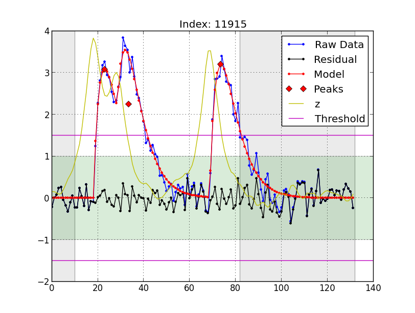
Each plot shows a single block. The following information is plotted:

• Raw Data is the data we'd like to fit with some number of pulses.
• Residual is the residual after the bset-fit pulses have been subtracted from Raw Data.
• Model is the best fit to the data that was obtained.
• Peaks mark the peak of each fit pulse.
• z is the output of the modified phase-only correlation (MPOC) algorithm used to initially identify the pulse positions. The min_denom parameter acts as a low-pass filter on z.
• Threshold is the th parameter.
• The green shaded region indicates the lowest amplitude pulse that will be fit, given by the parameter th_min.
• The grey shaded regions are the excluded regions. These are controled by exclude_pre and exclude_post.