slearn


A package linking symbolic representation with scikit-learn machine learning.
Symbolic representations of time series have proved their usefulness in the field of time series motif discovery, clustering, classification, forecasting, anomaly detection, etc. Symbolic time series representation methods do not only reduce the dimensionality of time series but also speedup the downstream time series task. It has been demonstrated by [S. Elsworth and S. Güttel, Time series forecasting using LSTM networks: a symbolic approach, arXiv, 2020] that symbolic forecasting has greatly reduce the sensitivity of hyperparameter settings for Long Short Term Memory networks. How to appropriately deploy machine learning algorithm on the level of symbols instead of raw time series poses a challenge to the interest of applications. To boost the development of research community on symbolic representation, we develop this Python library to simplify the process of machine learning algorithm practice on symbolic representation. slearn library provide different API for symbols generation associated with complexity measure and machine learining traning. We will illustrate several topics in detail as below.
Now let's get started!
Install the slearn package simply by
pip
pip install slearn
conda
conda install -c conda-forge slearn
To check which version you install, please use:
conda list slearn
Model support
slearn currently supports SAX, ABBA, and fABBA symbolic representation, and the machine learning classifiers as below:
| Support Classifiers | Parameter call |
|---|---|
| Multi-layer Perceptron | 'MLPClassifier' |
| K-Nearest Neighbors | 'KNeighborsClassifier' |
| Gaussian Naive Bayes | 'GaussianNB' |
| Decision Tree | 'DecisionTreeClassifier' |
| Support Vector Classification | 'SVC' |
| Radial-basis Function Kernel | 'RBF' |
| Logistic Regression | 'LogisticRegression' |
| Quadratic Discriminant Analysis | 'QuadraticDiscriminantAnalysis' |
| AdaBoost classifier | 'AdaBoostClassifier' |
| Random Forest | 'RandomForestClassifier' |
| LightGBM | 'LGBM' |
Our documentation is available.
Symbolic machine learning prediction
Import the package
from slearn import symbolicMLWe can predict any symbolic sequence by choosing the classifiers available in scikit-learn.
string = 'aaaabbbccd'
sbml = symbolicML(classifier_name="MLPClassifier", ws=3, random_seed=0, verbose=0)
x, y = sbml.encode(string)
pred = sbml.forecast(x, y, step=5, hidden_layer_sizes=(10,10), learning_rate_init=0.1)
print(pred) #  ['d', 'b', 'a', 'b', 'b']
Also, you can use it by passing into parameters of dictionary form
string = 'aaaabbbccd'
sbml = symbolicML(classifier_name="MLPClassifier", ws=3, random_seed=0, verbose=0)
x, y = sbml.encode(string)
params = {'hidden_layer_sizes':(10,10), 'activation':'relu', 'learning_rate_init':0.1}
pred = sbml.forecast(x, y, step=5, **params)
print(pred) # ['d', 'b', 'a', 'b', 'b'] # the prediction
The parameter settings for the chosen classifier follow the same as the scikit-learn library, so just ensure that parameters are existing in the scikit-learn classifiers. More details are refer to scikit-learn website.
Time series forecasting with symbolic representation
Load libraries.
import pandas as pd
import numpy as np
import seaborn as sns
import matplotlib.pyplot as plt
from slearn import *

time_series = pd.read_csv("Amazon.csv") # load the required dataset, here we use Amazon stock daily close price.
ts = time_series.Close.values
Set the number of symbols you would like to predict.
step = 50You can select the available classifiers and symbolic representation method (currently we support SAX, ABBA and fABBA) for prediction. Similarly, the parameters of the chosen classifier follow the same as the scikit-learn library. We usually deploy ABBA symbolic representation, since it achieves better forecasting against SAX.
slean leverages user-friendly API, time series forecasting follows:
-
Step 1: Define the windows size (features size), the forecasting steps, symbolic representation method (SAX, ABBA or fABBA) and classifier.
-
Step 2: Transform time series into symbols with user specified parameters defined for symbolic representation.
-
Step 3: Define the classifier parameters and forecast the future values.
Use Gaussian Naive Bayes method:
sl = slearn(method='fABBA',  ws=3, step=step, classifier_name="GaussianNB") # step 1
sl.set_symbols(series=ts, tol=0.01, alpha=0.2) # step 2
sklearn_params = {'var_smoothing':0.001} # step 3
abba_nb_pred = sl.predict(**sklearn_params) # step 3
For the last two lines, they can also be replaced with the alternative way in a clear form:
abba_nb_pred = sl.predict(var_smoothing=0.001) # step 3This follows the same as below.
Try neural network models method:
sl = slearn(method='fABBA', ws=3, step=step, classifier_name="MLPClassifier") # step 1
sl.set_symbols(series=ts, tol=0.01, alpha=0.2)  # step 2
sklearn_params = {'hidden_layer_sizes':(20,80), 'learning_rate_init':0.1} # step 3
abba_nn_pred = sl.predict(**sklearn_params) # step 3
Now we try to preduct real-world time series. We can plot the prediction and compare the results.
import pandas as pd
import numpy as np
import seaborn as sns
import matplotlib.pyplot as plt
from slearn import *
np.random.seed(0)

time_series = pd.read_csv("Amazon.csv")
ts = time_series.Close.values
length = len(ts)
train, test = ts[:round(0.9*length)], ts[round(0.9*length):]

sl = slearn(method='fABBA', ws=8, step=1000, classifier_name="GaussianNB")
sl.set_symbols(series=train, tol=0.01, alpha=0.1)
abba_nb_pred = sl.predict(var_smoothing=0.001)
sl = slearn(method='fABBA', ws=8, step=1000, classifier_name="DecisionTreeClassifier")
sl.set_symbols(series=train, tol=0.01, alpha=0.1)
abba_nn_pred = sl.predict(max_depth=10, random_state=0)
sl = slearn(method='fABBA', ws=8, step=1000, classifier_name="KNeighborsClassifier")
sl.set_symbols(series=train, tol=0.01, alpha=0.1)
abba_kn_pred = sl.predict(n_neighbors=10)
sl = slearn(method='fABBA', ws=8, step=100, classifier_name="SVC")
sl.set_symbols(series=train, tol=0.01, alpha=0.1)
abba_svc_pred = sl.predict(C=20)
min_len = np.min([len(test), len(abba_nb_pred), len(abba_nn_pred)])

plt.figure(figsize=(20, 5))
sns.set(font_scale=1.5, style="whitegrid")
sns.lineplot(data=test[:min_len], linewidth=6, color='k', label='ground truth')
sns.lineplot(data=abba_nb_pred[:min_len], linewidth=6, color='tomato', label='prediction (fABBA - GaussianNB)')
sns.lineplot(data=abba_nn_pred[:min_len], linewidth=6, color='m', label='prediction (fABBA - DecisionTreeClassifier)')
sns.lineplot(data=abba_nn_pred[:min_len], linewidth=6, color='c', label='prediction (fABBA - KNeighborsClassifier)')
sns.lineplot(data=abba_svc_pred[:min_len], linewidth=6, color='yellowgreen', label='prediction (fABBA - Support Vector Classification)')
plt.legend()
plt.tick_params(axis='both', labelsize=15)
plt.show()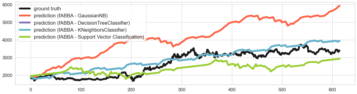
Flexible symbolic sequence generator
slearn library also contains functions for the generation of strings of tunable complexity using the LZW compressing method as base to approximate Kolmogorov complexity. This part of code is from https://github.com/robcah/RNNExploration4SymbolicTS, developed by Dr. Roberto Cahuantzi and Prof. Stefan Güttel.
from slearn import *
df_strings = LZWStringLibrary(symbols=3, complexity=[3, 9])
df_strings
Processing: 2 of 2
| nr_symbols | LZW_complexity | length | string | |
|---|---|---|---|---|
| 0 | 3 | 3 | 3 | BCA |
| 1 | 3 | 9 | 12 | ABCBBCBBABCC |
df_iters = pd.DataFrame()
for i, string in enumerate(df_strings['string']):
    kwargs = df_strings.iloc[i,:-1].to_dict()
    seed_string = df_strings.iloc[i,-1]
    df_iter = RNN_Iteration(seed_string, iterations=2, architecture='LSTM', **kwargs)
    df_iter.loc[:, kwargs.keys()] = kwargs.values()
    df_iters = df_iters.append(df_iter)
df_iter.reset_index(drop=True, inplace=True)
...
df_iters.reset_index(drop=True, inplace=True)
df_iters| jw | dl | total_epochs | seq_test | seq_forecast | total_time | nr_symbols | LZW_complexity | length | |
|---|---|---|---|---|---|---|---|---|---|
| 0 | 1.000000 | 1.0 | 12 | ABCABCABCA | ABCABCABCA | 2.685486 | 3 | 3 | 3 |
| 1 | 1.000000 | 1.0 | 14 | ABCABCABCA | ABCABCABCA | 2.436733 | 3 | 3 | 3 |
| 2 | 0.657143 | 0.5 | 36 | CBBCBBABCC | AABCABCABC | 3.352712 | 3 | 9 | 12 |
| 3 | 0.704762 | 0.4 | 36 | CBBCBBABCC | ABCBABBBBB | 3.811584 | 3 | 9 | 12 |
LZW compression
Lempel–Ziv–Welch (LZW) is a lossless data compression method created by Abraham Lempel, Jacob Ziv, and Terry Welch. Its simplicity makes it prevalent and universal nowadays. slearn provides a convenient API to easily implement the algorithm.
import slearn

string = 'abcabcdabcacbd'
compressed = slearn.LZWcompress(string)
decompressed = slearn.LZWdecompress(compressed)
print(string == decompressed)
Citation
If you use the function of LZWStringLibrary in your research, please cite:
@techreport{CCG21,
  title   = {{A comparison of LSTM and GRU networks for learning symbolic sequences}},
  author  = {Cahuantzi, Roberto and Chen, Xinye and G\"{u}ttel, Stefan},
  year    = {2021},
  number  = {arXiv:2107.02248},
  pages   = {12},
  institution = {The University of Manchester},
  address = {UK},
  type    = {arXiv EPrint},
  url     = {https://arxiv.org/abs/2107.02248}
}
License
This project is licensed under the terms of the MIT license.

Contributing
Contributing to this repo is welcome! We will work through all the pull requests and try to merge into main branch.

