som-pbc README

A simple self-organizing map implementation in Python with periodic boundary conditions.
Self-organizing maps are also called Kohonen maps and were invented by Teuvo Kohonen.[1] They are an unsupervised machine learning technique to efficiently create spatially organized internal representations of various types of data. For example, SOMs are well-suited for the visualization of high-dimensional data.
This is a simple implementation of SOMs in Python. This SOM has periodic
boundary conditions and therefore can be imagined as a "donut". The
implementation uses numpy, scipy, scikit-learn and
matplotlib.
Installation
som-pbc can be installed from pypi using pip:
pip install som-pbc
To upgrade som-pbc to the latest version, run:
pip install --upgrade som-pbc
Usage
Then you can import and use the SOM class as follows:
import numpy as np
from som import SOM
# generate some random data with 36 features
data1 = np.random.normal(loc=-.25, scale=0.5, size=(500, 36))
data2 = np.random.normal(loc=.25, scale=0.5, size=(500, 36))
data = np.vstack((data1, data2))
som = SOM(10, 10) # initialize a 10 by 10 SOM
som.fit(data, 10000, save_e=True, interval=100) # fit the SOM for 10000 epochs, save the error every 100 steps
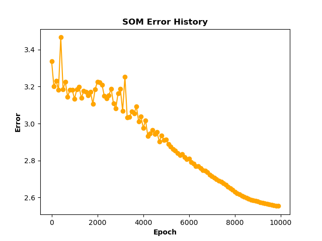
som.plot_error_history(filename='images/som_error.png') # plot the training error history
targets = np.array(500 * [0] + 500 * [1]) # create some dummy target values
# now visualize the learned representation with the class labels
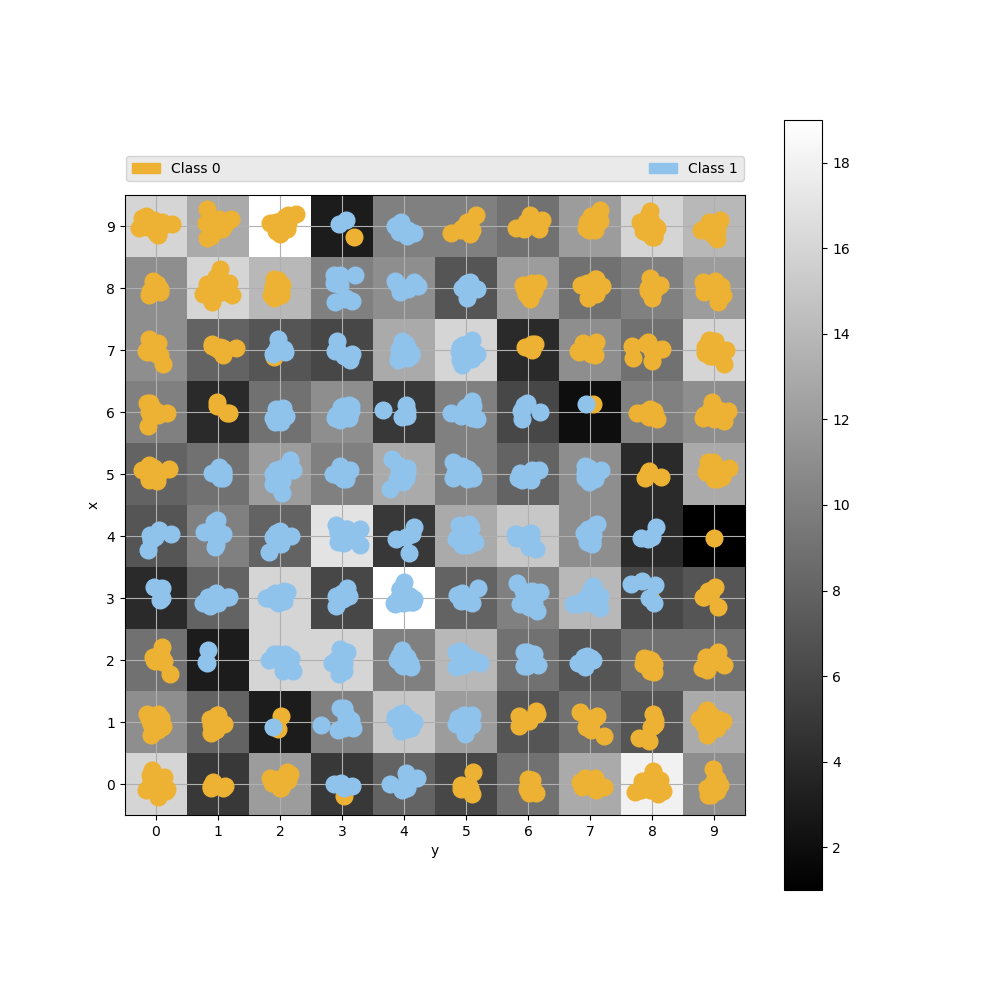
som.plot_point_map(data, targets, ['Class 0', 'Class 1'], filename='images/som.png')
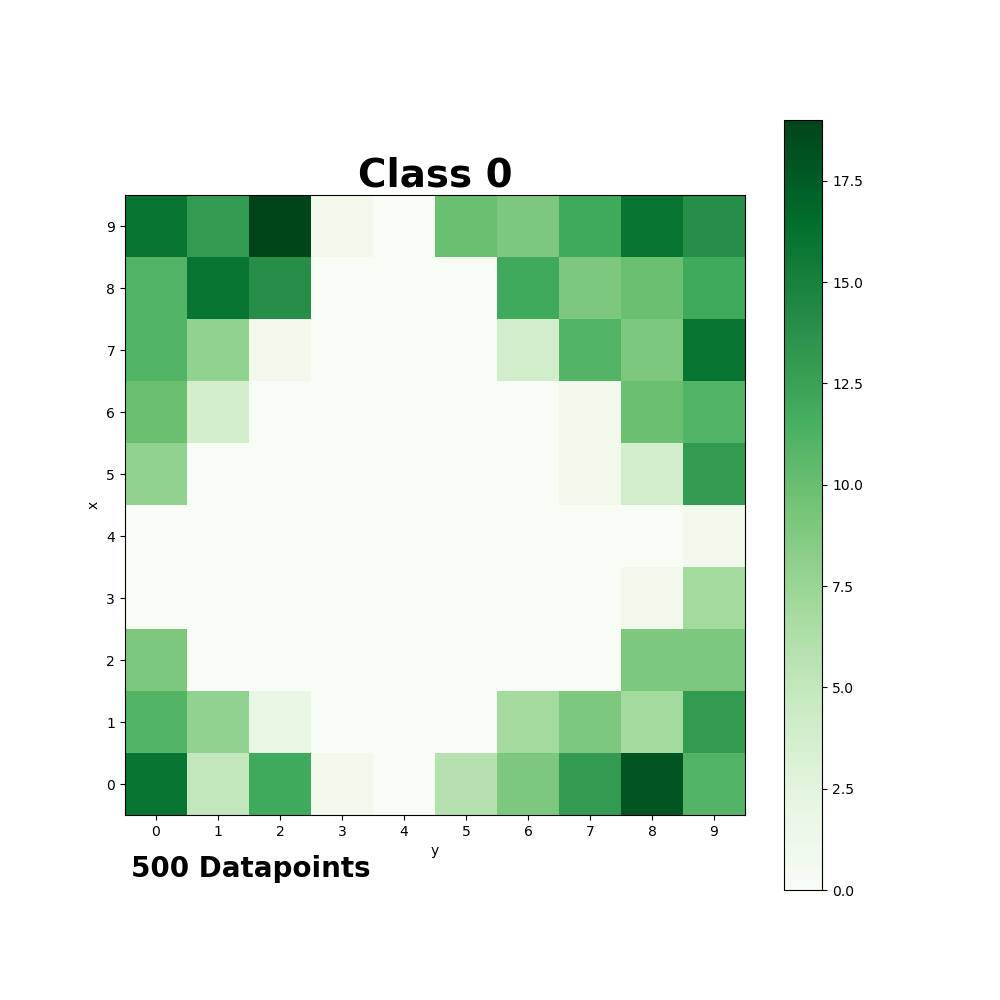
som.plot_class_density(data, targets, t=0, name='Class 0', colormap='Greens', filename='images/class_0.png')
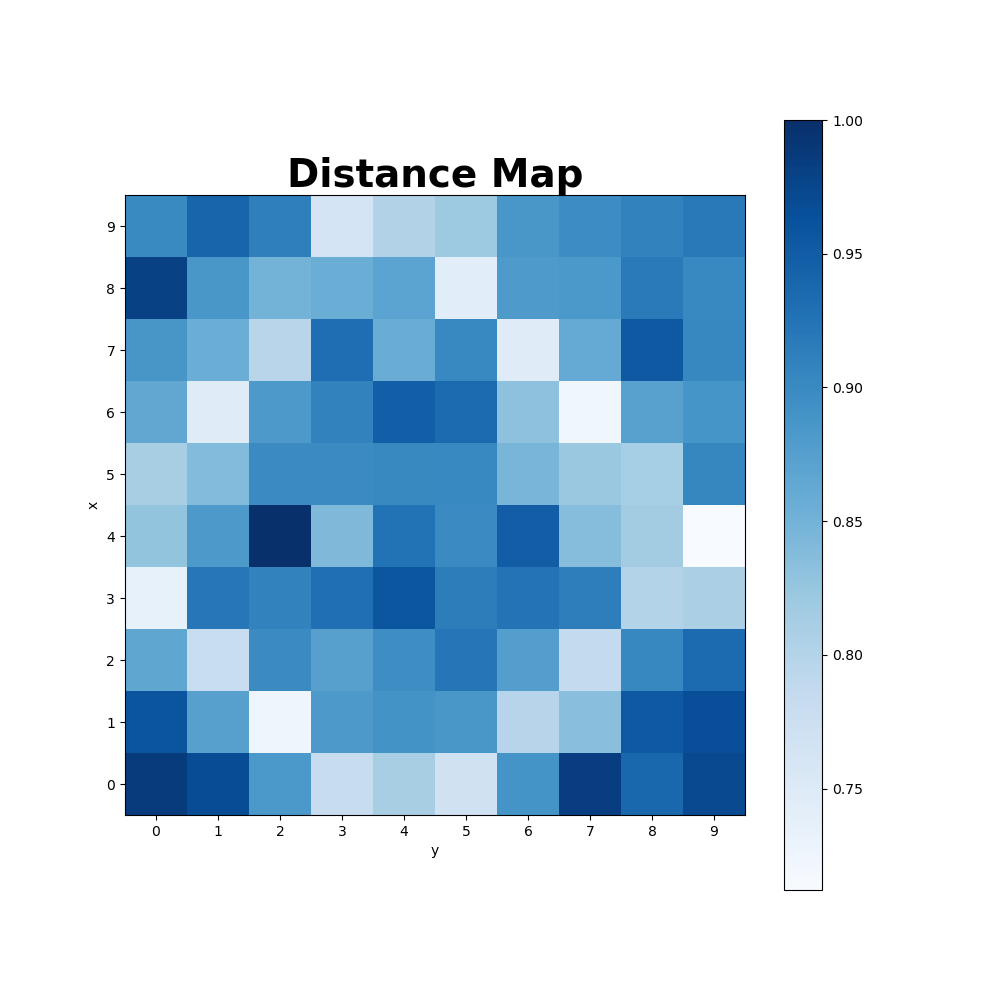
som.plot_distance_map(colormap='Blues', filename='images/distance_map.png') # plot the distance map after training
# predicting the class of a new, unknown datapoint
datapoint = np.random.normal(loc=.25, scale=0.5, size=(1, 36))
print("Labels of neighboring datapoints: ", som.get_neighbors(datapoint, data, targets, d=0))
# transform data into the SOM space
newdata = np.random.normal(loc=.25, scale=0.5, size=(10, 36))
transformed = som.transform(newdata)
print("Old shape of the data:", newdata.shape)
print("New shape of the data:", transformed.shape)Training Error:
Point Map:
Class Density:
Distance Map:
The same way you can handle your own data.
Methods / Functions
The SOM class has the following methods:
-
initialize(data, how='pca'): initialize the SOM, either via Eigenvalues (pca) or randomly (random) -
winner(vector): compute the winner neuron closest to a given data point invector(Euclidean distance) -
cycle(vector): perform one iteration in adapting the SOM towards the chosen data point invector -
fit(data, epochs=0, save_e=False, interval=1000, decay='hill'): train the SOM on the givendatafor severalepochs -
transform(data): transform givendatain to the SOM space -
distance_map(metric='euclidean'): get a map of every neuron and its distances to all neighbors based on the neuron weights -
winner_map(data): get the number of times, a certain neuron in the trained SOM is winner for the givendata -
winner_neurons(data): for every data point, get the winner neuron coordinates -
som_error(data): calculates the overall error as the average difference between the winning neurons and thedata -
get_neighbors(datapoint, data, labels, d=0): get the labels of alldataexamples that aredneurons away fromdatapointon the map -
save(filename): save the whole SOM instance into a pickle file -
load(filename): load a SOM instance from a pickle file -
plot_point_map(data, targets, targetnames, filename=None, colors=None, markers=None, density=True): visualize the som with all data as points around the neurons -
plot_density_map(data, filename=None, internal=False): visualize the data density in different areas of the SOM. -
plot_class_density(data, targets, t, name, colormap='Oranges', filename=None): plot a density map only for the given class -
plot_distance_map(colormap='Oranges', filename=None): visualize the disance of the neurons in the trained SOM -
plot_error_history(color='orange', filename=None): visualize the training error history after training (fit withsave_e=True)
References:
[1] Kohonen, T. Self-Organized Formation of Topologically Correct Feature Maps. Biol. Cybern. 1982, 43 (1), 59–69.
This work was partially inspired by ramalina's som implementation and JustGlowing's minisom.
Documentation:
Documentation for som-pbc is hosted on readthedocs.io.


