EZ2
Updated Python module implementation of the R package "EZ2" that accompanies the paper
Grasman, R. P. P. P., Wagenmakers, E.-J., & van der Maas, H. L. J. (2007). On the mean and variance of response times under the diffusion model with an application to parameter estimation, J. Math. Psych. 53: 55-68.
Example
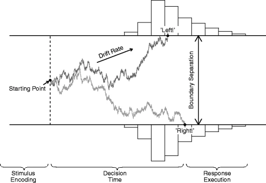
Consider the example of a lexical decision 2AFC response time task from the paper: There are 'word' and 'non-word' stimuli presented to subjects who have to indicate as quickly as possible whether the stimulus is a word or a non-word for many trials. As a result of such an experiment, for each subject we have
- a mean response time for 'words' (
mrt0) and a mean response time for 'non-words' (mrt1) - a variance of the response times for 'words' (
vrt0) and a variance of the response times for 'non-words' (vrt1) - a percentage of trials in which the subject made errors for 'words' (
pe0), and such a percentage for 'non-words' (pe1)
To estimate the parameters the EZ2 way (statistically known as Methods of Moments estimation), it turns out only the variances and error percentages are needed.
The EZ2 package is a lot more flexible than being applicable to just the above 2AFC type tasks. Effects of different types of stimuli may be hypothesized to lie in the drift rate, starting point, or boundary separation, or even the non-decision time component. That's why the model needs to be specified in terms of model equations in terms of relevant parameters.
For the lexical decision task example it is often hypothesized that the drift rate for 'words', denoted v0, is higher than the drift rate for non-words, v1. The carefulness of the subject is reflected in the boundary seperation parameter a, which is usually assumed to be constant across randomized trials (at least in the short run of the experiment). If 'words' stimuli occur more frequently than 'non-words' stimuli, subjects tend to be biased to anticipate a 'words' stimulus more than a 'non-words' stimulus, resulting in more error responses on 'non-words'. This is modeled as a shift of the starting point, often denoted z, to the boundary that corresponds to the 'words' response, and the same amount away from the 'non-words' boundary. If the starting point for the 'words' stimuli is given by z, the starting 'non-words' is therefore then given by a-z. The equations needed for this lexical decision task are therefore given by
-
vrt0is modeled asEZ2.vrt(v0, z, a) -
vrt1is modeled asEZ2.vrt(v1, a-z, a) -
pe0is modeled asEZ2.pe(v0, z, a) -
pe1is modeled asEZ2.pe(v1, a-z, a)
Generate data
First create some fake data. Data generated here are population variances and percentages of error responses for a number of sets of diffusion model parameter values. (This could correspond to different subjects having different values of v0, v1, z, and a.) In practice you would use of course estimated variances and error percentages for each subject from the recorded response times for each subject.
import pandas as pd
import EZ2

## create some data (theoretical values, not simulated) for a typic
## 2AFC experiment — in this example a lexical decision task
## (Needless to say, in reality you would moments computed from real data!)

# true parameter values (10 different cases)
par_df = pd.DataFrame({
     "v0": [0.1 + (0.3-0.1)*i/10 for i in range(11)],
     "v1": [0.15 + (0.4-0.15)*i/10 for i in range(11)],
     "z":  [0.15 + 0.03*(i-5)/5 for i in range(11)],
     "a":  [0.25]*11
 })

# compute the theoretical variance (vrt0) and proportion error (pe0) for
# the 'word' response times, and the theoretical variance (vrt1) and error
# (pe1) for the 'non-word' response times.
dat_df = pd.DataFrame({
    'vrt0': eval('EZ2.vrt(v0,z,a)', globals(), par_df),
    'pe0' : eval('EZ2.pe(v0,z,a)', globals(), par_df),
    'vrt1': eval('EZ2.vrt(v1,a-z,a)', globals(), par_df),
    'pe1' : eval('EZ2.pe(v1,a-z,a)', globals(), par_df)
 })
dat_df        # now pretend that `dat_df` is the data frame that
              # you have computed from real data; each row containing
              # vrt0, pe0, vrt1, and pe1 from a single participant
The parameters and data look like this:
print(pd.concat([par_df,dat_df],axis=1))| v0 | v1 | z | a | vrt0 | pe0 | vrt1 | pe1 | |
|---|---|---|---|---|---|---|---|---|
| 0 | 0.1 | 0.15 | 0.12 | 0.25 | 0.631635 | 0.0845497 | 0.283616 | 0.0196997 |
| 1 | 0.12 | 0.175 | 0.126 | 0.25 | 0.456897 | 0.0462423 | 0.203525 | 0.0128801 |
| 2 | 0.14 | 0.2 | 0.132 | 0.25 | 0.326752 | 0.0239326 | 0.149945 | 0.00887018 |
| 3 | 0.16 | 0.225 | 0.138 | 0.25 | 0.232702 | 0.0117509 | 0.113401 | 0.00646083 |
| 4 | 0.18 | 0.25 | 0.144 | 0.25 | 0.165954 | 0.00548281 | 0.087874 | 0.00498789 |
| 5 | 0.2 | 0.275 | 0.15 | 0.25 | 0.11902 | 0.00243346 | 0.0695974 | 0.00408571 |
| 6 | 0.22 | 0.3 | 0.156 | 0.25 | 0.0860831 | 0.00102804 | 0.0561972 | 0.00355256 |
| 7 | 0.24 | 0.325 | 0.162 | 0.25 | 0.0628774 | 0.000413546 | 0.0461548 | 0.00327962 |
| 8 | 0.26 | 0.35 | 0.168 | 0.25 | 0.0463874 | 0.000158435 | 0.0384793 | 0.00321474 |
| 9 | 0.28 | 0.375 | 0.174 | 0.25 | 0.034533 | 5.7814e-05 | 0.0325108 | 0.00334596 |
| 10 | 0.3 | 0.4 | 0.18 | 0.25 | 0.0258981 | 2.00936e-05 | 0.0278019 | 0.00369786 |
Run EZ2
Two options:
- easy with
ez2_2afcthat precisely suits the 2AFC experiment such as a lexical decision task - slightly more involve
EZ2that allows for more general models
Both are illustrated:
option 1
## recover the parameters from the pretend data `dat_df`: 2AFC experiments
EZ2.ez2_2afc(dat_df, ['vrt0','pe0','vrt1','pe1'], correct_only=False)
Here correct_only = False signifies that RT variances were compute from all the responses
regardless of correctness. See help(ez2_2afc) for more info. The output is similar as from option 2 below.
option 2
If the data doesn't exactly conform the lexical decision task set up, the more flexible way is as follows:
## recover the parameters from the pretend data `dat_df`: flexible way

# specify the model expressions for each column
column_models = [
     'vrt(v0,z,a)',        # first column: vrt0
     'pe(v0,z,a)',         # second column: pe0
     'vrt(v1,a-z,a)',      # third column: vrt1, starting point = a-z
     'pe(v1, a-z, a)']     # fourth column: pe1

# solve for parameters: try 16 random starting values for each row
pstart = {'v0': 0.17, 'v1': 0.15, 'z': 0.12, 'a': 0.25}

ez2fit = EZ2.batch(pstart, column_models, dat_df)
ez2fit
The result looks like this:
| v0 | v1 | z | a | niter | success | norm_error | message | |
|---|---|---|---|---|---|---|---|---|
| 0 | 0.1 | 0.15 | 0.12 | 0.25 | 18 | True | 7.76479e-12 | The solution converged. |
| 1 | 0.12 | 0.175 | 0.126 | 0.25 | 17 | True | 1.81379e-11 | The solution converged. |
| 2 | 0.14 | 0.2 | 0.132 | 0.25 | 17 | True | 1.09059e-12 | The solution converged. |
| 3 | 0.16 | 0.225 | 0.138 | 0.25 | 18 | True | 2.34994e-10 | The solution converged. |
| 4 | 0.18 | 0.25 | 0.144 | 0.25 | 18 | True | 4.71896e-12 | The solution converged. |
| 5 | 0.2 | 0.275 | 0.15 | 0.25 | 29 | True | 9.53827e-15 | The solution converged. |
| 6 | 0.22 | 0.3 | 0.156 | 0.25 | 27 | True | 1.13789e-14 | The solution converged. |
| 7 | 0.24 | 0.325 | 0.162 | 0.25 | 24 | True | 9.48528e-13 | The solution converged. |
| 8 | 0.26 | 0.35 | 0.168 | 0.25 | 33 | True | 5.90823e-12 | The solution converged. |
| 9 | 0.28 | 0.375 | 0.174 | 0.25 | 28 | True | 1.74185e-13 | The solution converged. |
| 10 | 0.3 | 0.4 | 0.18 | 0.25 | 36 | True | 1.79156e-14 | The solution converged. |
Comparison of columns v0, v1, z and a with the same colums from the true parameter values in the previous table, shows that the true parameter values are retrieved well.
See help(batch) or help(EZ2) for documentation of the available function.
List of function
| Description | |
|---|---|
| data2ez | Convert observed sample moments to parameter values of the 'EZ' drift diffusion process with absorbing boundaries 0 and a, starting at a/2. |
| cmrt, cvrt | Compute exit (decision) time mean and variance _conditional_ on exit through the bottom boundary (chosen alternative) of a diffusion process between absorbing boundaries. |
| mrt, vrt | Compute exit/decision time mean and variance irrespective of exit point (chosen alternative) |
| pe | Compute probability of exit through lower bound of a drift diffusion with constant drift |
| ez2_2afc | Fit simple drift diffusion model to observed sample moments of 2AFC task responses. Convenience wrapper function for EZ2(). |
| EZ2 | Fit a simple drift diffusion model to observed sample moments |
| batch | Batch EZ2 model fitting |
| pddexit | Cumulative distribution, density and quantile functions of exit times from top or bottom boundary of a drift diffusion process. |
| dddexit | Compute the density of exit times from top or bottom boundary of a drift diffusion process. |
| qddexit | Compute the quantiles for the cumulative distribution function of exit times from top or bottom boundary of a drift diffusion process. |
| rddexit | Generate random sample of exit times from top or bottom boundary of a drift diffusion process. |
| rddexitj | Generate random sample of exit times from top and bottom boundaries of a drift diffusion process. |
| ddexit_fit | Maximum likelihood estimation of parameters nu, z, a (and optionally an offset) of a constant drift diffusion process from the exit times of hitting either or both bounds. |
