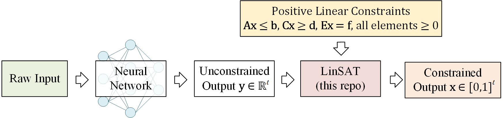
This is the official implementation of our ICML 2023 paper "LinSATNet: The Positive Linear Satisfiability Neural Networks".

• [paper]

With LinSATNet, you can enforce the satisfiability of general positive linear constraints to the output of neural networks.

LinSATNet supports sparse constraints starting v0.1.1! The forward and backward should be identical to the dense version, but the sparse version is expected to be more efficient in time and GPU memory. Upgrade by pip install --upgrade linsatnet

The LinSAT layer is fully differentiable, and the gradients are exactly computed. Our implementation now supports PyTorch.

You can install it by

pip install linsatnet

And get started by

from LinSATNet import linsat_layer

• LinSATNet
  • A Quick Example
  • API Reference
    • The linsat_layer function
    • Some practical notes
  • How it works?
    • Classic Sinkhorn with single-set marginals
    • Extended Sinkhorn with multi-set marginals
    • Transforming positive linear constraints into marginals
      • Encoding neural network's output
      • From linear constraints to marginals
  • More Complicated Use Cases (appeared in our paper)
    • I. Neural Solver for Traveling Salesman Problem with Extra Constraints
    • II. Partial Graph Matching with Outliers on Both Sides
    • III. Portfolio Allocation
  • Citation

There is a quick example if you run LinSATNet/linsat.py directly. In this example, the doubly-stochastic constraint is enforced for 3x3 variables.

To run the example, first clone the repo:

git clone https://github.com/Thinklab-SJTU/LinSATNet.git

Go into the repo, and run the example code:

cd LinSATNet
python LinSATNet/linsat.py

In this example, we try to enforce doubly-stochastic constraint to a 3x3 matrix. The doubly-stochastic constraint means that all rows and columns of the matrix should sum to 1.

The 3x3 matrix is flattened into a vector, and the following positive linear constraints are considered (for $\mathbf{E}\mathbf{x}=\mathbf{f}$):

E = torch.tensor(
    [[1, 1, 1, 0, 0, 0, 0, 0, 0],
     [0, 0, 0, 1, 1, 1, 0, 0, 0],
     [0, 0, 0, 0, 0, 0, 1, 1, 1],
     [1, 0, 0, 1, 0, 0, 1, 0, 0],
     [0, 1, 0, 0, 1, 0, 0, 1, 0],
     [0, 0, 1, 0, 0, 1, 0, 0, 1]], dtype=torch.float32
)
f = torch.tensor([1, 1, 1, 1, 1, 1], dtype=torch.float32)

We randomly init w and regard it as the output of some neural networks:

w = torch.rand(9) # w could be the output of neural network
w = w.requires_grad_(True)

We also have a "ground-truth target" for the output of linsat_layer, which is an diagonal matrix in this example:

x_gt = torch.tensor(
    [1, 0, 0,
     0, 1, 0,
     0, 0, 1], dtype=torch.float32
)

The forward/backward passes of LinSAT follow the standard PyTorch style and are readily integrated into existing deep learning pipelines.

The forward pass:

linsat_outp = linsat_layer(w, E=E, f=f, tau=0.1, max_iter=10, dummy_val=0)

The backward pass:

loss = ((linsat_outp - x_gt) ** 2).sum()
loss.backward()

You can also set E as a sparse matrix to improve the time & memory efficiency (especially for large-sized input):

linsat_outp = linsat_layer(w, E=E.to_sparse(), f=f, tau=0.1, max_iter=10, dummy_val=0)

We can also do gradient-based optimization over w to make the output of linsat_layer closer to x_gt. This is what's happening when you train a neural network.

niters = 10
opt = torch.optim.SGD([w], lr=0.1, momentum=0.9)
for i in range(niters):
    x = linsat_layer(w, E=E, f=f, tau=0.1, max_iter=10, dummy_val=0)
    cv = torch.matmul(E, x.t()).t() - f.unsqueeze(0)
    loss = ((x - x_gt) ** 2).sum()
    loss.backward()
    opt.step()
    opt.zero_grad()
    print(f'{i}/{niters}\n'
          f'  underlying obj={torch.sum(w * x)},\n'
          f'  loss={loss},\n'
          f'  sum(constraint violation)={torch.sum(cv[cv > 0])},\n'
          f'  x={x},\n'
          f'  constraint violation={cv}')

And you are likely to see the loss decreasing during the gradient steps.

To use LinSATNet in your own project, make sure you have the package installed:

pip install linsatnet

and import the pacakge at the beginning of your code:

from LinSATNet import linsat_layer, init_constraints

LinSATNet.linsat_layer(x, A=None, b=None, C=None, d=None, E=None, f=None, constr_dict=None, tau=0.05, max_iter=100, dummy_val=0, mode='v2', grouped=True, no_warning=False) [source]

LinSAT layer enforces positive linear constraints to the input x and projects it with the constraints $$\mathbf{A} \mathbf{x} <= \mathbf{b}, \mathbf{C} \mathbf{x} >= \mathbf{d}, \mathbf{E} \mathbf{x} = \mathbf{f}$$ and all elements in $\mathbf{A}, \mathbf{b}, \mathbf{C}, \mathbf{d}, \mathbf{E}, \mathbf{f}$ must be non-negative.

Parameters:

• x: PyTorch tensor of size ($n_v$), it can optionally have a batch size ($b \times n_v$)
• A, C, E: PyTorch tensor of size ($n_c \times n_v$), constraint matrix on the left hand side
• b, d, f: PyTorch tensor of size ($n_c$), constraint vector on the right hand side
• constr_dict: a dictionary with initialized constraint information, which is the output of the function LinSATNet.init_constraints. Specifying this variable could avoid re-initializing the constraints for the same constraints and improve the efficiency
• tau: (default=0.05) parameter to control the discreteness of the projection. Smaller value leads to more discrete (harder) results, larger value leads to more continuous (softer) results.
• max_iter: (default=100) max number of iterations
• dummy_val: (default=0) the value of dummy variables appended to the input vector
• mode: (default='v2') LinSAT kernel implementation. v1 is the one came with the ICML paper, v2 is the improved version with (usually) better efficiency
• grouped: (default=True) group non-overlapping constraints in one operation for better efficiency
• no_warning: (default=False) turn off warning message

return: PyTorch tensor of size ($n_v$) or ($b \times n_v$), the projected variables

Notations:

• $b$ means the batch size.
• $n_c$ means the number of constraints ($\mathbf{A}$, $\mathbf{C}$, $\mathbf{E}$ may have different $n_c$)
• $n_v$ means the number of variables

1. You must ensure that your input constraints have a non-empty feasible space. Otherwise, linsat_layer will not converge. It is also worth noting that x is in the range of [0, 1], and you may add a multiplier to scale it.
2. You may tune the value of tau for your specific tasks. Monitor the output of LinSAT so that the "smoothness" of the output meets your task. Reasonable choices of tau may range from 1e-4 to 100 in our experience.
3. Be careful of potential numerical issues. Sometimes A x <= 1 does not work, but A x <= 0.999 works.
4. The input vector x may have a batch dimension, but the constraints can not have a batch dimension. The constraints should be consistent for all data in one batch.
5. Input constraints as sparse tensors can usually help you save GPU memory. When working with sparse constraints, A, C, E should be torch.sparse_coo_tensor, and b, d, f should be dense tensors.

Here we introduce the mechanism inside LinSAT. It works by extending the Sinkhorn algorithm to multiple sets of marginals (to our best knowledge, we are the first to study Sinkhorn with multi-sets of marginals). The positive linear constraints are then enforced by transforming the constraints into marginals. For more details and formal proofs, please refer to our paper.

Let's start with the classic Sinkhorn algorithm. Given non-negative score matrix $\mathbf{S}\in\mathbb{R}_{\geq 0}^{m\times n}$ and a set of marginal distributions on rows $\mathbf{v}\in \mathbb{R}_{\geq 0}^m$ and columns $\mathbf{u} \in \mathbb{R}_{\geq 0}^n$, where $$\sum_{i=1}^m v_i = \sum_{j=1}^n u_j = h,$$ the Sinkhorn algorithm outputs a normalized matrix $\mathbf{\Gamma}\in[0,1]^{m\times n}$ so that $$\sum_{i=1}^m \Gamma_{i,j}u_{j}=u_j, \sum_{j=1}^n \Gamma_{i,j}u_{j}=v_i.$$ Conceptually, $\Gamma_{i,j}$ means the proportion of $u_j$ moved to $v_i$.

If you are seeing the math formulas not rendered correctly, it is an issue of github. Please refer to our main paper for better view.

The algorithm steps are:

Initialize $\Gamma_{i,j}=\frac{s_{i,j}}{\sum_{i=1}^m s_{i,j}}$

$\quad$repeat:

$\qquad{\Gamma}_{i,j}^{\prime} = \frac{{\Gamma}_{i,j}v_{i}}{\sum_{j=1}^n {\Gamma}_{i,j}u_{j}}$; $\triangleright$ normalize w.r.t. $\mathbf{v}$

$\qquad{\Gamma}_{i,j} = \frac{{\Gamma}_{i,j}^{\prime}u_{j}}{\sum_{i=1}^m {\Gamma}_{i,j}^{\prime}u_{j}}$; $\triangleright$ normalize w.r.t. $\mathbf{u}$

$\quad$until convergence.

Note that the above formulation is modified from the conventional Sinkhorn formulation. $\Gamma_{i,j}u_j$ is equivalent to the elements in the "transport" matrix in papers such as (Cuturi 2013). We prefer this new formulation as it generalize smoothly to Sinkhorn with multi-set marginals in the following.

To make a clearer comparison, the transportation matrix in (Cuturi 2013) is $\mathbf{P}\in\mathbb{R}_{\geq 0}^{m\times n}$, and the constraints are $$\sum_{i=1}^m P_{i,j}=u_{j},\quad \sum_{j=1}^n P_{i,j}=v_{i}$$ $P_{i,j}$ means the exact mass moved from $u_{j}$ to $v_{i}$.

The algorithm steps are:

Initialize $\Gamma_{i,j}=\frac{s_{i,j}}{\sum_{i=1}^m s_{i,j}}$

$\quad$repeat:

$\qquad{P}_{i,j}^{\prime} = \frac{P_{i,j}v_{i}}{\sum_{j=1}^n {P}_{i,j}}$; $\triangleright$ normalize w.r.t. $\mathbf{v}$

$\qquad{P}_{i,j} = \frac{{P}_{i,j}^{\prime}u_j}{\sum_{i=1}^m {P}_{i,j}^{\prime}}$; $\triangleright$ normalize w.r.t. $\mathbf{u}$

$\quad$until convergence.

We discover that the Sinkhorn algorithm can generalize to multiple sets of marginals.

Recall that $\Gamma_{i,j}\in[0,1]$ means the proportion of $u_i$ moved to $v_j$. Interestingly, it yields the same formulation if we simply replace $\mathbf{u},\mathbf{v}$ by another set of marginal distributions, suggesting the potential of extending the Sinkhorn algorithm to multiple sets of marginal distributions. Denote that there are $k$ sets of marginal distributions that are jointly enforced to fit more complicated real-world scenarios. The sets of marginal distributions are $\mathbf{u}_\eta\in \mathbb{R}_{\geq 0}^n, \mathbf{v}_\eta\in \mathbb{R}_{\geq 0}^m$, and we have: $$\forall \eta\in {1, \cdots,k}: \sum_{i=1}^m v_{\eta,i}=\sum_{j=1}^n u_{\eta,j}=h_\eta.$$

It assumes the existence of a normalized $\mathbf{Z} \in [0,1]^{m\times n}$ s.t. $$\forall \eta\in {1,\cdots, k}: \sum_{i=1}^m z_{i,j} u_{\eta,j}=u_{\eta,j}, \sum_{j=1}^n z_{i,j} u_{\eta,j}=v_{\eta,i}$$ i.e., the multiple sets of marginal distributions have a non-empty feasible region (you may understand the meaning of "non-empty feasible region" after reading the next section about how to handle positive linear constraints). Multiple sets of marginal distributions could be jointly enforced by traversing the Sinkhorn iterations over $k$ sets of marginal distributions.

The algorithm steps are:

Initialize $\Gamma_{i,j}=\frac{s_{i,j}}{\sum_{i=1}^m s_{i,j}}$

$\quad$repeat:

$\qquad$for $\eta=1$ to $k$ do

$\quad\qquad{\Gamma}_{i,j}^{\prime} = \frac{{\Gamma}_{i,j}v_{\eta,i}}{\sum_{j=1}^n {\Gamma}_{i,j}u_{\eta,j}}$; $\triangleright$ normalize w.r.t. $\mathbf{v}_\eta$

$\quad\qquad{\Gamma}_{i,j} = \frac{{\Gamma}_{i,j}^{\prime}u_{\eta,j}}{\sum_{i=1}^m {\Gamma}_{i,j}^{\prime}u_{\eta,j}}$; $\triangleright$ normalize w.r.t. $\mathbf{u}_\eta$

$\qquad$end for

$\quad$until convergence.

In our paper, we prove that the Sinkhorn algorithm for multi-set marginals shares the same convergence pattern with the classic Sinkhorn, and its underlying formulation is also similar to the classic Sinkhorn.

Then we show how to transform the positive linear constraints into marginals, which are handled by our proposed multi-set Sinkhorn.

For an $l$-length vector denoted as $\mathbf{y}$ (which can be the output of a neural network, also it is the input to linsat_layer), the following matrix is built

$\mathbf{W} = {y}_1 \quad {y}_2 \quad ... \quad {y}_l \quad \beta$

$\qquad \ \ \beta \ \quad \beta \ \quad ... \quad \ \beta \quad \ \beta$

where $\mathbf{W}$ is of size $2 \times (l+1)$, and $\beta$ is the dummy variable, the default is $\beta=0$. $\mathbf{y}$ is put at the upper-left region of $\mathbf{W}$. The entropic regularizer is then enforced to control discreteness and handle potential negative inputs: $$\mathbf{S} = \exp \left(\frac{\mathbf{W}}{\tau}\right).$$

The score matrix $\mathbf{S}$ is taken as the input of Sinkhorn for multi-set marginals.

• Packing constraint $\mathbf{A}\mathbf{x}\leq \mathbf{b}$. Assuming that there is only one constraint, we rewrite the constraint as $$\sum_{i=1}^l a_ix_i \leq b.$$ Following the "transportation" view of Sinkhorn, the output $\mathbf{x}$ moves at most $b$ unit of mass from $a_1, a_2, \cdots, a_l$, and the dummy dimension allows the inequality by moving mass from the dummy dimension. It is also ensured that the sum of $\mathbf{u}_p$ equals the sum of $\mathbf{v}_p$. The marginal distributions are defined as

• Covering constraint $\mathbf{C}\mathbf{x}\geq \mathbf{d}$. Assuming that there is only one constraint, we rewrite the constraint as $$\sum_{i=1}^l c_ix_i\geq d.$$ We introduce the multiplier $$\gamma=\left\lfloor\sum_{i=1}^lc_i / d \right\rfloor$$ because we always have $$\sum_{i=1}^l c_i \geq d$$ (else the constraint is infeasible), and we cannot reach the feasible solution where all elements in $\mathbf{x}$ are 1s without this multiplier. Our formulation ensures that at least $d$ unit of mass is moved from $c_1, c_2, \cdots, c_l$ by $\mathbf{x}$, thus representing the covering constraint of "greater than". It is also ensured that the sum of $\mathbf{u}_c$ equals the sum of $\mathbf{v}_c$. The marginal distributions are defined as

• Equality constraint $\mathbf{E}\mathbf{x}= \mathbf{f}$. Representing the equality constraint is more straightforward. Assuming that there is only one constraint, we rewrite the constraint as $$\sum_{i=1}^l e_ix_i= f.$$ The output $\mathbf{x}$ moves $e_1, e_2, \cdots, e_l$ to $f$, and we need no dummy element in $\mathbf{u}_e$ because it is an equality constraint. It is also ensured that the sum of $\mathbf{u}_e$ equals the sum of $\mathbf{v}_e$. The marginal distributions are defined as

After encoding all constraints and stack them as multiple sets of marginals, we can call the Sinkhorn algorithm for multi-set marginals to enforce the constraints.

The Traveling Salesman Problem (TSP) is a classic NP-hard problem. The standard TSP aims at finding a cycle visiting all cities with minimal length, and developing neural solvers for TSP receives increasing interests. Beyond standard TSP, here we develop a neural solver for TSP with extra constraints using LinSAT layer.

Contributing author: Yunhao Zhang

To run the TSP experiment, please follow the code and instructions in TSP_exp/.

Standard graph matching (GM) assumes an outlier-free setting namely bijective mapping. One-shot GM neural networks (Wang et al., 2022) effectively enforce the satisfiability of one-to-one matching constraint by single-set Sinkhorn. Partial GM refers to the realistic case with outliers on both sides so that only a partial set of nodes are matched. There lacks a principled approach to enforce matching constraints for partial GM. The main challenge for existing GM networks is that they cannot discard outliers because the single-set Sinkhorn is outlier-agnostic and tends to match as many nodes as possible. The only exception is BBGM (Rolinek et al., 2020) which incorporates a traditional solver that can reject outliers, yet its performance still has room for improvement.

Contributing author: Ziao Guo

To run the GM experiment, please follow the code and instructions in ThinkMatch/LinSAT.

Predictive portfolio allocation is the process of selecting the best asset allocation based on predictions of future financial markets. The goal is to design an allocation plan to best trade-off between the return and the potential risk (i.e. the volatility). In an allocation plan, each asset is assigned a non-negative weight and all weights should sum to 1. Existing learning-based methods (Zhang et al., 2020), (Butler et al., 2021) only consider the sum-to-one constraint without introducing personal preference or expert knowledge. In contrast, we achieve such flexibility for the target portfolio via positive linear constraints: a mix of covering and equality constraints, which is widely considered for its real-world demand.

Contributing author: Tianyi Chen

To run the portfolio experiment, please follow the code and instructions in portfolio_exp/.

If you find our paper/code useful in your research, please cite

@inproceedings{WangICML23,
  title={{LinSATNet}: The Positive Linear Satisfiability Neural Networks},
  author={Wang, Runzhong and Zhang, Yunhao and Guo, Ziao and Chen, Tianyi and Yang, Xiaokang and Yan, Junchi},
  booktitle={International Conference on Machine Learning (ICML)},
  year={2023}
}