Create your own insured portfolio using several Tools.
First ,To install, just use pip :
pip install pyinsuranceRequired Dependencies are listed below , such :
| Dependency | Version |
|---|---|
| arch | 5.0.1 |
| numpy | 1.20.1 |
| scipy | 1.6.2 |
| statsmodels | 0.12.2 |
| numba | 0.52.1 |
| setuptools | 60.5.0 |
| pandas | 1.2.4 |
There is no dependency verification , so please, make sure to have installed every required one before using the package.
Example
To begin, let’s extract some included default data :
import pyinsurance
from pyinsurance.pymolder import tipp_model
from pyinsurance.data.IRX import load as d1
from pyinsurance.data.sp500 import load as d2
import matplotlib.pyplot as plt

risky_Asset = d2()
safe_Asset = d1()/52  #we divided by 52 as we use weekly rates
Let’s initalise our first insured portfolio now!
For instance,we set our lock-in rate , minimum capital risk allocation , threshold for capital injection , allocate funds ,strategy’s percentage floor ,multipler,benchmark returns and rebalancement cycle being respectively equal to :
lock_in_rate = 0.05
mcr = 0.40
tfci = 0.80
fund = 100
floor = 0.80
multiplier = 10
Benchmark_return = risk_Asset
Rebalancement_frequency = 52 # once a week -> 52 weeks a year
Running the tipp_model class :
res = tipp_model(risk_Asset,safe_Asset,lock_in_rate,mcr,tfci,fund,\
                floor,multiplier,risk_Asset,Rebalancement_frequency)
Our strategy-insured backtest is ready !
import matplotlib.pyplot as plt
from pyinsurance.Metric_Generator.returns_metrics import Cumulative_ret


fig = plt.figure(figsize=(15,5))
ax0 = fig.add_subplot(111)
plt.plot(risk_Asset.index,Cumulative_ret(risk_Asset)*100,label = 'Non-Insured Performance')
plt.plot(risk_Asset.index,res.Fund,label = 'Fund Performance')
plt.plot(risk_Asset.index,res.Reference_capital,label = 'Reference Capital',linestyle="--")
plt.plot(risk_Asset.index,res.floor,label = 'Floor',linestyle="-.")
plt.legend()
plt.show()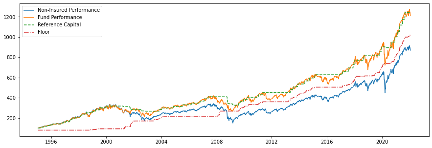
And our capital injections through the period are presented as:
fig = plt.figure(figsize=(15,5))
ax1 = fig.add_subplot(111)
plt.plot(risk_Asset.index,res.capital_reinjection,label = 'Injected Capital')
plt.legend()
plt.show()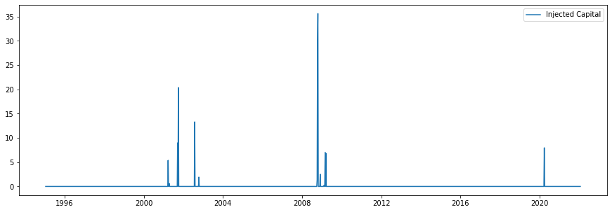
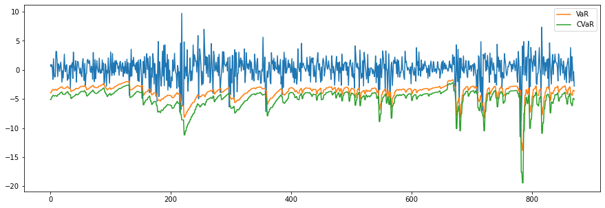
If you want to backtest the VaR, you can use the varpy library: