Bayesian Hidden Markov Models


This code implements a non-parametric Bayesian Hidden Markov model, sometimes referred to as a Hierarchical Dirichlet Process Hidden Markov Model (HDP-HMM), or an Infinite Hidden Markov Model (iHMM). This package has capability for a standard non-parametric Bayesian HMM, as well as a sticky HDPHMM (see references). Inference is performed via Markov chain Monte Carlo estimation, including efficient beam sampling for the latent sequence resampling steps, and multithreading when possible for parameter resampling.
Installation
The current version is development only, and installation is only recommended for people who are aware of the risks. It can be installed through PyPI:
pip install bayesian-hmmHidden Markov Models
Hidden Markov Models
are powerful time series models, which use latent variables to explain observed emission sequences.
The result is a generative model for time series data, which is often tractable and can be easily understood.
The latent series is assumed to be a Markov chain, which requires a starting distribution and transition distribution,
as well as an emission distribution to tie emissions to latent states.
Traditional parametric Hidden Markov Models use a fixed number of states for the latent series Markov chain.
Hierarchical Dirichlet Process Hidden Markov Models (including the one implemented by bayesian_hmm package) allow
for the number of latent states to vary as part of the fitting process.
This is done by using a hierarchical Dirichlet prior on the latent state starting and transition distributions,
and performing MCMC sampling on the latent states to estimate the model parameters.
Usage
Basic usage allows us to supply a list of emission sequences, initialise the HDPHMM, and perform MCMC estimation. The below example constructs some artificial observation series, and uses a brief MCMC estimation step to estimate the model parameters. We use a moderately sized data to showcase the speed of the package: 50 sequences of length 200, with 500 MCMC steps.
import bayesian_hmm

# create emission sequences
base_sequence = list(range(5)) + list(range(5, 0, -1))
sequences = [base_sequence * 20 for _ in range(50)]

# initialise object with overestimate of true number of latent states
hmm = bayesian_hmm.HDPHMM(sequences, sticky=False)
hmm.initialise(k=20)

results = hmm.mcmc(n=500, burn_in=100, ncores=3, save_every=10, verbose=True)
This model typically converges to 10 latent states, a sensible posterior. In some cases, it converges to 11 latent states, in which a starting state which outputs '0' with high confidence is separate to another latent start which outputs '0' with high confidence. We can inspect this using the printed output, or with probability matrices printed directly.
# print final probability estimates (expect 10 latent states)
hmm.print_probabilities()
This final command prints the transition and emission probabiltiies of the model after
MCMC using the terminaltables package. The
code below visualises the results using pandas
and seaborn. For simplicity, we will stick with
the returned MAP estimate, but a more complete analysis might use a more sophisticated
approach.
import pandas as pd
import seaborn as sns
import matplotlib.pyplot as plt
plt.style.use('ggplot')

# plot the number of states as a histogram
sns.countplot(results['state_count'])
plt.title('Number of latent states')
plt.xlabel('Number of latent states')
plt.ylabel('Number of iterations')
plt.show()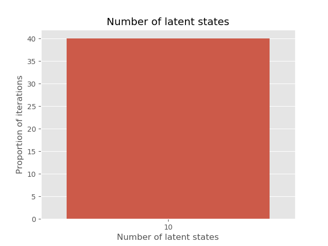
# plot the starting probabilities of the sampled MAP estimate
map_index = results['chain_loglikelihood'].index(min(results['chain_loglikelihood']))
parameters_map = results['parameters'][map_index]
sns.barplot(
    x=list(parameters_map['p_initial'].keys()),
    y=list(parameters_map['p_initial'].values())
)
plt.title('Starting state probabilities')
plt.xlabel('Latent state')
plt.ylabel('MAP estimate for initial probability')
plt.show()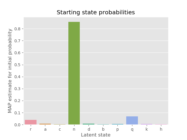
# convert list of hyperparameters into a DataFrame
hyperparam_posterior_df = (
    pd.DataFrame(results['hyperparameters'])
    .reset_index()
    .melt(id_vars=['index'])
    .rename(columns={'index': 'iteration'})
)
hyperparam_prior_df = pd.concat(
    pd.DataFrame(
        {'iteration': range(500), 'variable': k, 'value': [v() for _ in range(500)]}
    )
    for k, v in hmm.priors.items()
)
hyperparam_df = pd.concat(
    (hyperparam_prior_df, hyperparam_posterior_df),
    keys=['prior', 'posterior'],
    names=('type','index')
)
hyperparam_df.reset_index(inplace=True)

# advanced: plot sampled prior & sampled posterior together
g = sns.FacetGrid(
    hyperparam_df[hyperparam_df['variable'] != 'kappa'],
    col='variable',
    col_wrap=3,
    sharex=False,
    hue='type'
)
g.map(sns.distplot, 'value')
g.add_legend()
g.fig.suptitle('Hyperparameter prior & posterior estimates')
plt.subplots_adjust(top=0.9)
plt.xlabel('Value')
plt.ylabel('Density')
plt.show()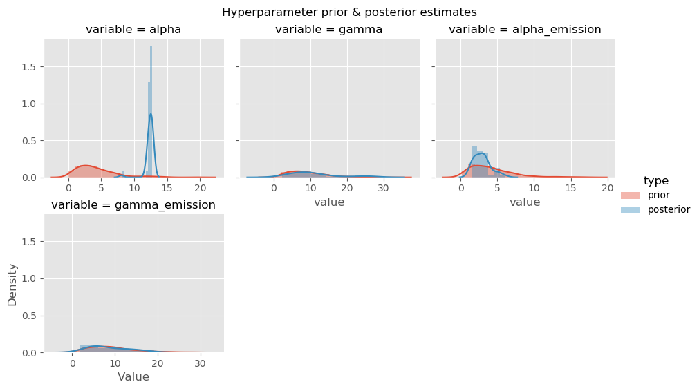
The bayesian_hmm package can handle more advanced usage, including:
- Multiple emission sequences,
- Emission series of varying length,
- Any categorical emission distribution,
- Multithreaded MCMC estimation, and
- Starting probability estimation, which share a dirichlet prior with the transition probabilities.
Inference
This code uses an MCMC approach to parameter estimation. We use efficient Beam sampling on the latent sequences, as well as Metropolis Hastings sampling on each of the hyperparameters. We approximate true resampling steps by using probability estimates calculated on all states of interest, rather than the leaving probabilities unadjusted for current variable resampling steps (rather than removing the current) variable for the sampled estimate.
Outstanding issues and future work
We have the following set as a priority to improve in the future:
- Expand package to include standard non-Bayesian HMM functions, such as Baum Welch and Viterbi algorithm
- Allow for missing or
NULLemissions which do not impact the model probability - Include functionality to use maximum likelihood estimates for the hyperparameters (currently only Metropolis Hastings resampling is possible for hyperparameters)
References
Van Gael, J., Saatci, Y., Teh, Y. W., & Ghahramani, Z. (2008, July). Beam sampling for the infinite hidden Markov model. In Proceedings of the 25th international conference on Machine learning (pp. 1088-1095). ACM.
Beal, M. J., Ghahramani, Z., & Rasmussen, C. E. (2002). The infinite hidden Markov model. In Advances in neural information processing systems (pp. 577-584).
Fox, E. B., Sudderth, E. B., Jordan, M. I., & Willsky, A. S. (2007). The sticky HDP-HMM: Bayesian nonparametric hidden Markov models with persistent states. Arxiv preprint.

