flowpy 💾 - A python package for working with optical flows

Optical flow is the displacement map of pixels between two frames. It is a low-level analysis used in many computer vision programs.

Working with optical flow may be cumbersome:

• It is quite hard to represent it in a comprehensible manner.
• Multiple formats exist for storing it.

Flowpy provides tools to work with optical flow more easily in python.

Installing

We recommend using pip:

pip install flowpy

Features

The main features of flowpy are:

• Reading and writing optical flows in two formats:
  • .flo (as defined here)
  • .png (as defined here)
• Visualizing optical flows with matplotlib
• Backward and forward warp

Examples

A simple RGB plot

This is the simplest example of how to use flowpy, it:

• Reads a file using flowpy.flow_read.
• Transforms the flow as an rgb image with flowpy.flow_to_rgb and shows it with matplotlib

Code:

import flowpy
import matplotlib.pyplot as plt

flow = flowpy.flow_read("tests/data/kitti_occ_000010_10.flo")

fig, ax = plt.subplots()
ax.imshow(flowpy.flow_to_rgb(flow))
plt.show()

Result:

Sample image from the KITTI dataset

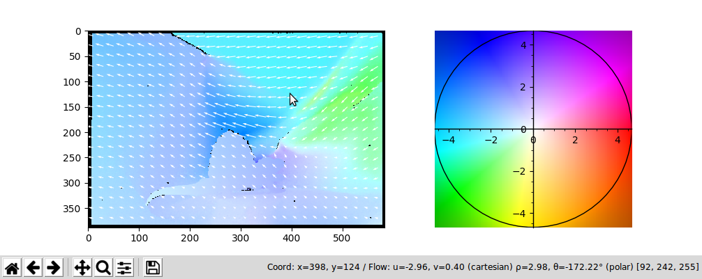
Plotting arrows, showing flow values and a calibration pattern

Flowpy comes with more than just RGB plots, the main features here are: - Arrows to quickly visualize the flow - The flow values below cursor showing in the tooltips - A calibration pattern side by side as a legend for your graph

Code:

flow = flowpy.flow_read("tests/data/Dimetrodon.flo")
height, width, _ = flow.shape

image_ratio = height / width
max_radius = flowpy.get_flow_max_radius(flow)

fig, (ax_1, ax_2) = plt.subplots(
    1, 2, gridspec_kw={"width_ratios": [1, image_ratio]}
)

ax_1.imshow(flowpy.flow_to_rgb(flow))
flowpy.attach_arrows(ax_1, flow)
flowpy.attach_coord(ax_1, flow)

flowpy.attach_calibration_pattern(ax_2, flow_max_radius=max_radius)

plt.show()

Result:

Sample image from the Middlebury dataset

Warping images (backward):

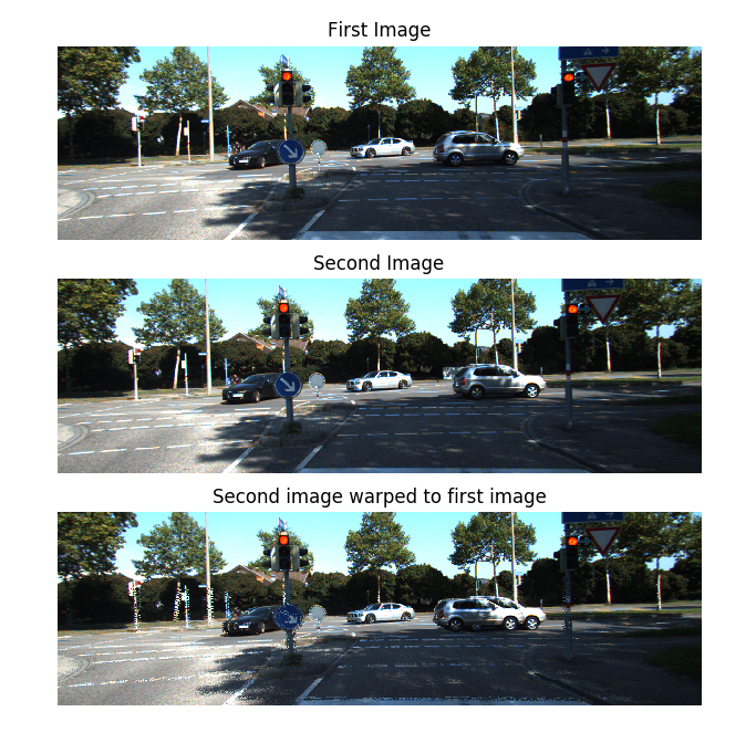
If you know the flow (first_image -> second_image), you can backward warp the second_image back to first_image.

flow = flowpy.flow_read("static/kitti_occ_000010_10.png")
first_image = np.asarray(Image.open("static/kitti_000010_10.png"))
second_image = np.asarray(Image.open("static/kitti_000010_11.png"))

flow[np.isnan(flow)] = 0
warped_first_image = flowpy.backward_warp(second_image, flow)

fig, axes = plt.subplots(3, 1)
for ax, image, title in zip(axes, (first_image, second_image, warped_first_image),
                            ("First Image", "Second Image", "Second image warped to first image")):
    ax.imshow(image)
    ax.set_title(title)
    ax.set_axis_off()

plt.show()

Result:

Note that the artifacts in the warp are normal, they are caused by unknown flows and occlusions.

Warping images (forward):

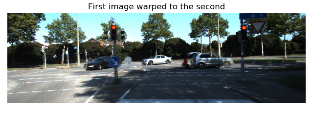
Forward warp is often less used as it is quite more complex. It relies on a k-nearest neighbor search instead of direct bi-linear interpolation.

forward_warp is about 10x slower than backward_warp but you still may find it useful.

flow = flowpy.flow_read("static/kitti_occ_000010_10.png")
first_image = np.asarray(Image.open("static/kitti_000010_10.png"))
second_image = np.asarray(Image.open("static/kitti_000010_11.png"))

flow[np.isnan(flow)] = 0
warped_second_image = flowpy.forward_warp(first_image, flow)

fig, ax = plt.subplots()

ax.imshow(warped_second_image)
ax.set_title( "First image warped to the second")
ax.set_axis_off()

plt.show()

Result:

More

You can find the above examples in the examples folder. You can also look in tests. If you encounter a bug or have an idea for a new feature, feel free to open an issue.

Most of the visualization and io handling has been translated from matlab and c code from the Middlebury flow code. Credits to thank Simon Baker, Daniel Scharste, J. P. Lewis, Stefan Roth, Michael J. Black and Richard Szeliski.