About
Basic image analysis tools, with the following functions:
-
imcrop(): image cropping, with interactive options, -
contour_properties(): calculate centroid, area, and perimeter of a contour, -
closest_contour(): closest contour to a position, -
contour_coords(): transform contour from scikit-image or opencv into usable x, y data,
The imgbasics.transform module also contains functions mimicking those found in Scikit Image's transform module, but that are based on OpenCV for improved speed. For now it only contains:
-
transform.rotate(): rotate image
Note: the package also defines a ContourError class as a custom exception for errors in contour calculations.
Install
pip install imgbasicsQuick start
Below is some information to use available functions. Please also consult docstrings and the Jupyter notebooks ExamplesBasics.ipynb for more details and examples.
Image cropping (imcrop)
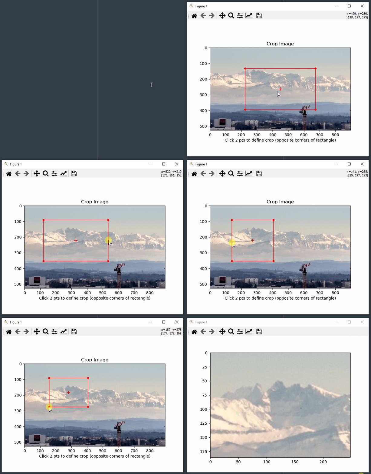
Image cropping function; the interactive mode allows the user to define the region of interest on the image interactively, either using clicks or a draggable rectangle.
The image img is assumed to be already loaded in memory as a numpy array (or equivalent, i.e. that supports slicing and defines shape and ndim attributes)
Non-interactive mode
img_crop = imgbasics.imcrop(img, cropzone)Crops the image img according to a pre-defined crop rectangle cropzone = xmin, ymin, width, height. Contrary to the Matlab imcrop function with the same name, the cropped image is really of the width and height requested in terms of number of pixels, not w+1 and h+1 as in Matlab.
Interactive mode
img_crop, cropzone = imgbasics.imcrop(img)Cropping rectangle is drawn on the image (img) by either:
- defining two corners of the rectangle by clicking (default).
- using a draggable rectangle for selection and pressing "enter" (
draggable=Trueoption)
The returned cropzone corresponds to xmin, ymin, width, height.
Note: when selecting, the pixels taken into account are those which have their centers closest to the click, not their edges closest to the click. For example, to crop to a single pixel, one needs to click two times within this pixel (possibly at the same location). For images with few pixels, this results in a visible offset between the dotted lines plotted after the clicks (running through the centers of the pixels clicked) and the final rectangle, which runs along the edges of all pixels selected.
Other arguments
Other arguments are available, e.g. for appearance, visibility, axes, etc. of the cropping tools. See docstrings for details.
Contour properties (contour_properties)
Returns centroid position, perimeter and area of a contour as a dictionary with keys 'centroid' (tuple with x and y position), 'perimeter' (positive float), 'area' (signed float). The sign convention for the area A differs depending on what type of plot is used (because plt.imshow() and plt.plot() do not use the same coordinate conventions):
| direction | imshow image (plt.imshow()) |
regular plot (plt.plot()) |
|---|---|---|
| clockwise | A < 0 | A > 0 |
| anti-clockwise | A > 0 | A < 0 |
(see ExamplesBasics.ipynb for a discussion of the direction of the contours returned by both scikit-image and opencv in different situations).
Example (Hexagon which rotates anti-clockwise in regular coordinates and clockwise on an imshow plot):
import numpy as np
from imgbasics import contour_properties

l = 1 / np.sqrt(3)
xp = np.array([1, 1, 0, -1, -1, 0])/2
yp = np.array([-l, l, 2*l, l, -l, -2*l])/2

data = contour_properties(xp, yp)
should return
data['centroid'] ~ (0, 0)
data['perimeter'] = 6 / sqrt(3) ~ 3.4641,
data['area'] = -sqrt(3)/2 ~ -0.8660
Closest contour (closest_contour)
Finds the closest contour (within a list of contours obtained by scikit-image or opencv) to a certain position (tuple (x, y)). Example with the example.png image provided in the package (should select the lowest, bright spot)
from skimage import io, measure
from imgbasics import closest_contour

img = io.imread('example.png')
contours = measure.find_contours(img, 170)

c = closest_contour(contours, (221, 281), edge=True, source='scikit')- If
edge = True, returns the contour with the edge closest to the position - If
edge = False(default), returns the contour with the average position closest to position. -
sourceis the origin of the contours ('scikit' or 'opencv')
Note: raises a ContourError if no contours in image (contours empty).
Contour coordinates (contour_coords)
Following the analysis in the section above (contour c), the contour_coords() function allow to format the contour into directly usable x, y coordinates for plotting directly on the imshow() image. For example, following the code above:
import matplotlib.pyplot as plt
from imgbasics import contour_coords

x, y = contour_coords(c, source='scikit')

fig, ax = plt.subplots()
ax.imshow(img, cmap='gray')
ax.plot(x, y, -r)
Image transformation module (imgbasics.transform)
This module mimicks Scikit Image's transform module but with calculations based on OpenCV for order-of-magnitude improvement (typically more than 10-fold) in speed. Right now it only contains the rotate() function.
from imgbasics.transform import rotate
from skimage import io

img = io.imread('example.png')
img_rot = rotate(img, angle=-23, resize=True, order=3)  # bicubic interpolation
Interactive cropping demo
With clicks (default):
With a draggable rectangle:
Dependencies
- python >= 3.6
- matplotlib
- numpy
- importlib-metadata
- drapo >= 1.2.0
-
[optional] openCV (cv2), only if using the
imgbasics.transformmodule (not listed in the install dependencies of theimgbasicspackage)
Author
Olivier Vincent
License
BSD 3-clause (see LICENSE file)

