ktransit
A simple exoplanet transit modeling tool in python

This python package contains routines to create and/or fit a transiting planet model. The underlying model is a Fortran implementation of the [Mandel & Agol (2002)] (http://iopscience.iop.org/1538-4357/580/2/L171/fulltext/16756.text.html) limb darkened transit model. The code will calculate a full orbital model and eccentricity can be allowed to vary.
With version 0.1, radial velocity data can now be calcaulted via the model and included in the fit
Installation
Install via pip
pip install ktransit
or via the git repository
git clone https://github.com/mrtommyb/ktransit.git
cd ktransit
python setup.py install
Making a model
The basic module, ktransit, will create a transit model. The code uses sensible defaults and only changes parameters explicitly stated. For example, to create a simple model just run
import ktransit
import matplotlib.pyplot as plt

M = ktransit.LCModel()
M.add_star()
M.add_planet()
M.add_data()

tmod = M.transitmodel
plt.plot(M.time,tmod)
of if you'd just prefer to see an Earth-like transit model then run
time,earthlc = ktransit.give_me_earth()
plt.plot(time,earthlc)
Now, the code allows the user to input their own parameters.
import ktransit
import matplotlib.pyplot as plt
import numpy

M = ktransit.LCModel()
M.add_star(
        rho=1.5, # mean stellar density in cgs units
        ld1=0.2, # ld1--4 are limb darkening coefficients
        ld2=0.4, # if only ld1 and ld2 are non-zero then a quadratic limb darkening law is used
        ld3=0.0, # if all four parameters are non-zero we use non-linear flavour limb darkening
        ld4=0.0,
        dil=0.0, # a dilution factor: 0.0 -> transit not diluted, 0.5 -> transit 50% diluted
        zpt=0.0  # a photometric zeropoint, incase the normalisation was wonky
        )
M.add_planet(
        T0=1.0,     # a transit mid-time
        period=1.0, # an orbital period in days
        impact=0.1, # an impact parameter
        rprs=0.1,   # planet stellar radius ratio
        ecosw=0.0,  # eccentricity vector
        esinw=0.0,
        occ=0.0)    # a secondary eclipse depth in ppm

M.add_planet() # you can add as many planets as you like (up to 10)

M.add_data(
        time=numpy.arange(0,10,0.0188),                                 # timestamps to evaluate the model on
        itime=numpy.zeros_like(numpy.arange(0,10,0.0188))+0.0188 )      # integration time of each timestamp

tmod = M.transitmodel # the out of transit data will be 0.0 unless you specify zpt
plt.plot(M.time,tmod)
Fitting
This is the fun part!! Fit a transit model to data. I use the scipy Levenberg–Marquardt least-squares minimization You need to give the model an initial guess and tell it what parameters you want to allow to vary, everything else is kept fixed.
The code assumes that the observed data has been normalised and detrended. The default zeropoint is 0.0 so the out of transit data should have a mean of 0.0 unless you want to change the zpt parameter.
A simple fitting example, there is no transit in the fake data I create here.
from ktransit import FitTransit

time = np.arange(0,10,0.0188)           # you need a time and a flux
flux = np.zeros_like(time)              # there are no transits here :(
ferr = np.ones_like(time) * 0.00001     # uncertainty on the data

fitT = FitTransit()
fitT.add_guess_star(rho=7.0)
fitT.add_guess_planet(
        period=365.25, impact=0.0,
        T0=0.0, rprs=0.009155)
fitT.add_data(time=time, flux=flux, ferr=ferr)

vary_star = ['rho', 'zpt']      # free stellar parameters
vary_planet = (['period',       # free planetary parameters
        'T0', 'impact',
        'rprs'])                # free planet parameters are the same for every planet you model

fitT.free_parameters(vary_star, vary_planet)
fitT.do_fit()                   # run the fitting

fitT.print_results()            # print some results
Best-fitting stellar parameters
rho: 5.02680657221
Best-fitting planet parameters for planet 0
impact: 0.0803742216248
period: 1.00000143821
T0: 1.49999092263
rprs: 0.0999846857972
Best-fitting planet parameters for planet 1
impact: 0.387103707996
period: 1.2000614885
T0: 0.700001081846
rprs: 0.0198908445261
The above comes from fitting a model with two planets in.
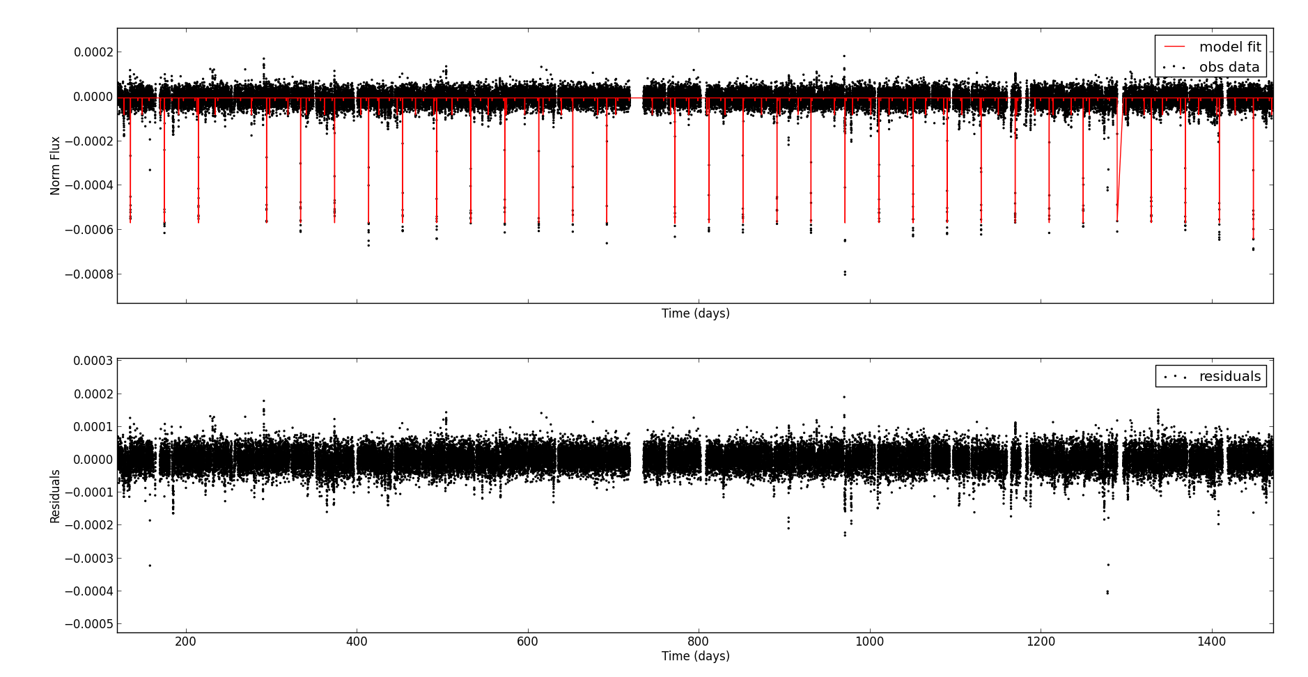
You can make a pretty plot of the output of the fitting by running
fig = ktransit.plot_results(time,flux,fitT.transitmodel)
fig.savefig('my_beautiful_fit.png') # or fig.show()
The plot below shows a three planet model fit to the Kepler-37 data. This plot can be created using the code in examples/
Including radial velocity data
New in version 0.1, you can now include radial velocity data.
import ktransit
import matplotlib.pyplot as plt
import numpy

M = ktransit.LCModel()
M.add_star(
        rho=1.5,
        ld1=0.2,
        ld2=0.4,
        ld3=0.0,
        ld4=0.0,
        dil=0.0,
        zpt=0.0,
        veloffset=10 # new keyword, the radial velocity zero-point offset in m/s
        )
M.add_planet(
        T0=1.0,
        period=1.0,
        impact=0.1,
        rprs=0.1,
        ecosw=0.0,
        esinw=0.0,
        occ=0.0,
        rvamp=100.) # radial velocity semi-amplitude in m/s

M.add_data(
        time=numpy.arange(0,10,0.0188),
        itime=numpy.zeros_like(numpy.arange(0,10,0.0188))+0.0188 )

M.add_rv(rvtime=numpy.arange(0,10,2.),                             # radial velocity observation timestamps
        rvitime=numpy.zeros_like(numpy.arange(0,10,2.))+0.02 )    # integration time of each timestamp

tmod = M.transitmodel
rvmodel = M.rvmodel
plt.plot(M.time,tmod)
plt.plot(M.rvtime,rvmodel)

