Mitty is a data simulator meant to help debug aligners and variant callers.

It requires Python 3.4 or later. It is released under the Apache license.

Features

• Generate reads from the whole genome, a single tiny region or from a set of regions as desired
• Handles X, Y chromosomes and polyploidy IF the VCF GT field is properly set
• Read qname stores correct POS, CIGAR and the sizes of variants covered by the read
• Name of sample included in read allowing us to mix FASTQs from different simulations/sources
  • Can mix viral contamination into reads
  • Can do tumor/normal mixes
• Corruption module adds sequencing errors to reads
  • Read models can be sampled from existing BAM files
• "God aligner" writes out a BAM with perfect alignments which can be used for BAM comparisons
• Simple genome simulator to generate VCFs with SNPs and different sizes of Insertions and Deletions for aligner/caller testing

It is also informative to browse the release notes and poke around the detailed documentation under the /docs folder

Quickstart

Install

conda create -n mymitty python=3.5

• Using a virtual env is recommended, but it's a personal choice
• Mitty requires Python3 to run

Install Mitty from the public github repository. Requires pip 9.0 or later

pip install --upgrade setuptools pip
pip install git+https://github.com/sbg/Mitty.git

Run tests

nosetests mitty.test -v

Program help

Help is available from the command line. Simply invoking the base program with no arguments will list all the sub programs with some short help:

mitty

Detailed help on particular commands is also available:

mitty generate-reads --help

Running commands with the verbose option allows you to tune what messages (ranging from Errors to Debug) you get.

mitty -v{1,2,3,4} <command>

Detailed tutorial with commentary

Example scripts and data

If you want to follow along with this tutorial you will find the relevant example scripts and test data in the https://github.com/kghosesbg/mitty-demo-data project.

The separate project has been created to avoid making the main source tree bulky by filling it with binary files not needed for program operation.

(Some of the examples require other tools such as samtools, bwa and vcftools)

Generating reads

(Example script)

Aliases used

FASTA=../data/human_g1k_v37.fa.gz
SAMPLEVCF=../data/1kg.20.22.vcf.gz
SAMPLENAME=HG00119
REGION_BED=region.bed
FILTVCF=HG00119-filt.vcf.gz
READMODEL=1kg-pcr-free.pkl
COVERAGE=30
READ_GEN_SEED=7
FASTQ_PREFIX=HG00119-reads
READ_CORRUPT_SEED=8

Prepare VCF file for taking reads from

The read simulator can not properly generate ground truth reads from overlapping variants (e.g. a deletion that overlaps a SNP on the same chromosome copy), complex variants (variant calls where the REF and ALT are both larger than 1 bp) or any entry that does not precisely lay out the ALT sequence in the ALT column, such as angle bracket ID references and variants breakend notation. Such calls must be filtered from a VCF file before it can be used as a sample to generate reads from.

mitty -v4 filter-variants \
  ${SAMPLEVCF} \
  ${SAMPLENAME} \
  ${REGION_BED} \
  - \
  2> vcf-filter.log | bgzip -c > ${FILTVCF}

tabix -p vcf ${FILTVCF}

The region.bed file is used to select out just the parts of the VCF we would like to generate reads from. The input VCF can be a population VCF (say from the 1000G project). The ${SAMPLENAME} indicates which sample to extract from the VCF.

vcf-filter.log looks like::

$ cat vcf-filter.log 
DEBUG:mitty.lib.vcfio:Starting filtering ...
DEBUG:mitty.lib.vcfio:Filtering ('1', 1000000, 2000000)
DEBUG:mitty.lib.vcfio:Complex variant 1:1827835 CTT -> ('CT', 'C')
DEBUG:mitty.lib.vcfio:Filtering ('3', 60830384, 61830384)
DEBUG:mitty.lib.vcfio:Complex variant 3:60835995 TTCTCTCTCTCTCTCTCTCTCTC -> ('TTCTCTCTCTCTCTCTCTCTCTCTCTCTC', 'T')
DEBUG:mitty.lib.vcfio:Complex variant 3:60897726 TAC -> ('TACAC', 'T')
DEBUG:mitty.lib.vcfio:Complex variant 3:60970457 GGTGTGT -> ('GGT', 'G')
DEBUG:mitty.lib.vcfio:Complex variant 3:61205001 ATG -> ('ATGTG', 'A')
DEBUG:mitty.lib.vcfio:Complex variant 3:61309628 GGTGTGTGTGTGTGTGT -> ('GGTGTGTGTGTGTGTGTGTGT', 'G')
DEBUG:mitty.lib.vcfio:Complex variant 3:61360782 AGTGTGTGTGT -> ('AGTGTGTGTGTGT', 'A')
DEBUG:mitty.lib.vcfio:Complex variant 3:61469726 CAAAAAAAAAAAAAAA -> ('CA', 'C')
DEBUG:mitty.lib.vcfio:Complex variant 3:61488707 TTGTG -> ('TTG', 'T')
DEBUG:mitty.lib.vcfio:Complex variant 3:61509647 TCACACACACA -> ('TCACACACACACACA', 'T')
DEBUG:mitty.lib.vcfio:Complex variant 3:61522251 TACACAC -> ('TACAC', 'T')
DEBUG:mitty.lib.vcfio:Complex variant 3:61541525 CA -> ('CAAA', 'C')
DEBUG:mitty.lib.vcfio:Complex variant 3:61633465 CAAAAAAA -> ('CAAAAAAAAAAAAA', 'C')
DEBUG:mitty.lib.vcfio:Complex variant 3:61718383 AAAATAAAT -> ('AAAAT', 'A')
DEBUG:mitty.lib.vcfio:Complex variant 3:61731724 CTTT -> ('CTT', 'C')
DEBUG:mitty.lib.vcfio:Processed 2807 variants
DEBUG:mitty.lib.vcfio:Sample had 2807 variants
DEBUG:mitty.lib.vcfio:Discarded 15 variants
DEBUG:mitty.lib.vcfio:Took 0.28023505210876465 s

NOTE: If the BED file is not sorted, the output file needs to be sorted again.

${FILTVCF} can now be used to generate reads and will serve as a truth VCF for VCF benchmarking.

Listing and inspecting read models

mitty list-read-models will list built in read models

mitty list-read-models -d ./mydir will list additional custom models stored in mydir

mitty describe-read-model 1kg-pcr-free.pkl model.png prints a panel of plots showing read characteristics

See later for a list of read models supplied with Mitty and their characteristics

Creating custom read models

This is only needed if none of the existing read models match your requirements

Prepare a Illumina type read model from a BAM

(Example script)

BAM=../data/sample.bam
MODELNAME=sampled-model.pkl

mitty -v4 create-read-model bam2illumina \
  --every 10 \
  --min-mq 20 \
  -t 2 \
  --max-bp 300 \
  --max-tlen 1000 \
  ${BAM} \
  ${MODELNAME} \
  'Sampled model created for the demo'

mitty describe-read-model ${MODELNAME} ${MODELNAME}.png

Create arbitrary Illumina type read models

The read model file is just a Python pickle file of a dictionary carrying specifications for the model. You can create arbitrary models by specifying your own parameters. Please see the read model documentation for a description of all the parameters.

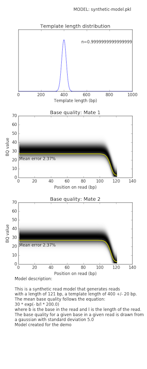
Easily prepare completely synthetic Illumina type read model

(Example script)

Mitty also supplies a model generator (synth-illumina) to generate custom Illumina like read models with template sizes and base quality patterns following simple mathematical distributions. This model generator allows us to quickly create reads models with a wide variety of independently variable parameters.

MODELNAME=synthetic-model.pkl

mitty create-read-model synth-illumina \
  ${MODELNAME} \
  --read-length 121 \
  --mean-template-length 400 \
  --std-template-length 20 \
  --bq0 30 \
  --k 200 \
  --sigma 5 \
  --comment 'Model created for the demo' \

The generated read model looks like:

Generating perfect reads

mitty -v4 generate-reads \
  ${FASTA} \
  ${FILTVCF} \
  ${SAMPLENAME} \
  ${REGION_BED} \
  ${READMODEL} \
  ${COVERAGE} \
  ${READ_GEN_SEED} \
  >(gzip > ${FASTQ_PREFIX}1.fq.gz) \
   ${FASTQ_PREFIX}-lq.txt \
   --fastq2 >(gzip > ${FASTQ_PREFIX}2.fq.gz) \
   --threads 2

(When you supply a model file name to the read generator it will first look among the builtin read models to see if the file name is a match (typically these are in the mitty/data/readmodels folder). It will then treat the model file name as a path and try and load that from your file system - which is the case in this particular example.)

The produced FASTQs have qnames encoding the correct read alignments for each read in the template. qnames may exceed the SAM specification limit (nominally 254 characters, but there are caveats). In such cases the qname in the FASTQ is truncated and the complete qname is printed in the side-car file ${FASTQ_PREFIX}-lq.txt.

The qname format can be obtained by executing mitty qname

Reference reads

As you might expect, by passing a VCF with no variants we can generate reads with no variants, representing the reference genome. One Mitty feature to be aware of is ploidy inference from the VCF: if there are no variants in a contig, Mitty assumes that contig is diploid, otherwise Mitty uses the GT (genotype) tag to infer ploidy.

(Example script)

Hence for a human male we set up the VCF (human-m-ref.vcf) as:

##fileformat=VCFv4.2
##FILTER=<ID=PASS,Description="All filters passed">
##fileDate=20160824
##contig=<ID=1,length=249250621>
##contig=<ID=2,length=243199373>
...
##contig=<ID=X,length=155270560>
##contig=<ID=Y,length=59373566>
##contig=<ID=MT,length=16569>
##FORMAT=<ID=GT,Number=1,Type=String,Description="Consensus Genotype across all datasets with called genotype">
#CHROM  POS     ID      REF     ALT     QUAL    FILTER  INFO    FORMAT  ref
X       1       .       A       G       50      PASS    .       GT      0
Y       1       .       A       G       50      PASS    .       GT      0

When we generate reads from this VCF say from chromosome 1, X and Y we see the following trace:

DEBUG:mitty.lib.vcfio:Contig: 1, ploidy: 2 (Assumed. Contig was empty)
DEBUG:mitty.lib.vcfio:Contig: X, ploidy: 1 
DEBUG:mitty.lib.vcfio:Contig: Y, ploidy: 1 

which tells us that contig 1 has been assumed to be diploid, whereas X and Y are inferred to be haploid because of the dummy entries we set.

(Example script)

Technically the human female VCF could be set up as a VCF with just the header (Mitty would infer all contigs to be diploid), but it turns out that some tools (including pysam) operate incorrectly when the VCF is completely empty, so we supply one dummy line for the VCF (human-f-ref.vcf) as:

##fileformat=VCFv4.2
##FILTER=<ID=PASS,Description="All filters passed">
##fileDate=20160824
##contig=<ID=1,length=249250621>
##contig=<ID=2,length=243199373>
...
##contig=<ID=X,length=155270560>
##contig=<ID=Y,length=59373566>
##contig=<ID=MT,length=16569>
##FORMAT=<ID=GT,Number=1,Type=String,Description="Consensus Genotype across all datasets with called genotype">
#CHROM  POS     ID      REF     ALT     QUAL    FILTER  INFO    FORMAT  ref
X       1       .       A       G       50      PASS    .       GT      0/0

Truncating reads

(Example script)

For some experiments you might want to generate custom sized reads. generate-reads allows you to do this with the --truncate-to argument

FASTQ_PREFIX=HG00119-truncated-reads
mitty -v4 generate-reads \
  ${FASTA} \
  ${FILTVCF} \
  ${SAMPLENAME} \
  ${REGION_BED} \
  ${READMODEL} \
  ${COVERAGE} \
  ${READ_GEN_SEED} \
  >(gzip > ${FASTQ_PREFIX}1.fq.gz) \
  ${FASTQ_PREFIX}-lq.txt \
  --fastq2 >(gzip > ${FASTQ_PREFIX}2.fq.gz) \
  --truncate-to 60 \
  --threads 2

This generates the same kind of reads as before, but all the reads are 60bp long, instead of their usual length. You can not make reads longer than what the model originally specifies (This to ensure that the read corruption code will work seamlessly with such truncated reads.)

Un-pairing reads

(Example script)

For some experiments you might want to use the existing Illumina or other model that normally produces paired-end reads to generate single-end reads instead. The --unpair argument allows you to do this. Note that in this case you should not pass in a second output FASTQ file.

FASTQ_PREFIX=HG00119-unpaired-reads
mitty -v4 generate-reads \
  ${FASTA} \
  ${FILTVCF} \
  ${SAMPLENAME} \
  ${REGION_BED} \
  ${READMODEL} \
  ${COVERAGE} \
  ${READ_GEN_SEED} \
  >(gzip > ${FASTQ_PREFIX}.fq.gz) \
   ${FASTQ_PREFIX}-lq.txt \
   --unpair \
   --threads 2

Flat-coverage

(Example script)

Adding the --flat-coverage flag will generate reads such that, excepting anomalies around the start and stop of the region, we obtain absolutely uniform coverage across the whole region. Template lengths still follow the distribution found in the model.

This is useful for a variety of experiments where variability in coverage if a metric.

Corrupting reads

The reads generated using the previous command have no base call errors. Base call errors can be introduced into the reads using the following command.

mitty -v4 corrupt-reads \
  ${READMODEL} \
  ${FASTQ_PREFIX}1.fq.gz >(gzip > ${FASTQ_PREFIX}-corrupt1.fq.gz) \
  ${FASTQ_PREFIX}-lq.txt \
  ${FASTQ_PREFIX}-corrupt-lq.txt \
  ${READ_CORRUPT_SEED} \
  --fastq2-in ${FASTQ_PREFIX}2.fq.gz \
  --fastq2-out >(gzip > ${FASTQ_PREFIX}-corrupt2.fq.gz) \
  --threads 2

Using a read model different to that used to generate the reads originally can lead to undefined behavior, including crashes.

As mentioned, the side-car file ${FASTQ_PREFIX}-lq.txt carries qnames longer than 254 characters. The output side-car file ${FASTQ_PREFIX}-corrupt-lq.txt similarly carries longer qnames from the corrupted reads. The qname for each corrupted template is identical to the original, uncorrupted template, except for the addition of an MD-like tag that allows recovery of the original bases before sequencing errors were introduced.

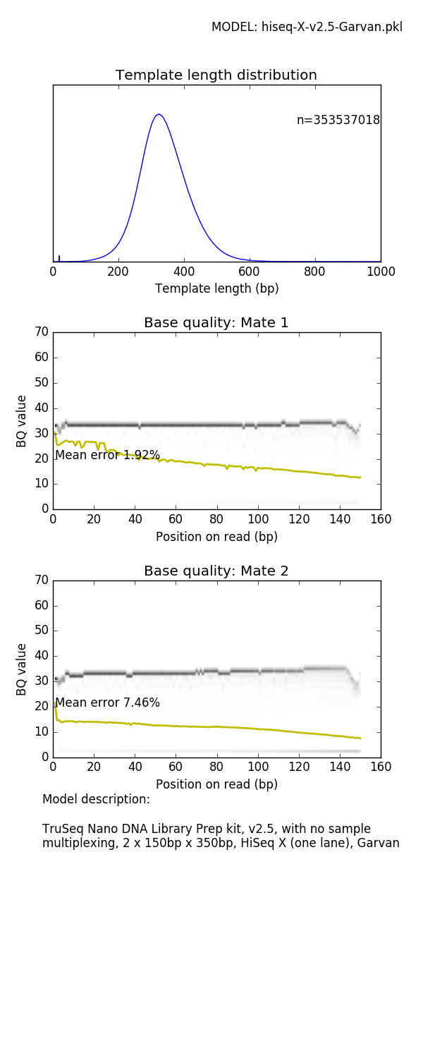
The BQ profile of the sample FASTQ generated by this command (generated by FASTQC) looks like

Mate 1:

Mate 2:

can be compared with the empirical model profile shown in the Appendix for the 1kg-pcr-free.pkl model.

After passing these reads through an aligner and viewing them on a genome browser, such as IGV one can make a quick inspection of the alignments.

Since the qname carries the correct alignment and CIGAR string you can match that against the actual alignment and CIGAR string for spot checks.

Perfect BAM (God aligner)

(Example script)

Passing the simulated FASTQ through the god aligner produces a "perfect BAM" which can be used as a truth BAM for comparing alignments from different aligners. This truth BAM can also be used to test variant callers by removing one moving part (the aligner) from the analysis chain.

FASTA=../data/human_g1k_v37.fa.gz
FASTQ_PREFIX=../generating-reads/HG00119-reads
GODBAM=HG00119-god.bam

mitty -v4 god-aligner \
  ${FASTA} \
  ${FASTQ_PREFIX}-corrupt1.fq.gz \
  ${FASTQ_PREFIX}-corrupt-lq.txt \
  ${GODBAM} \
  --fastq2 ${FASTQ_PREFIX}-corrupt2.fq.gz \
  --threads 2

Analysis tools library

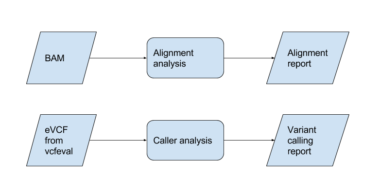
BAM analysis

Mitty provides tools (mitty.analysis) for analysing BAMs derived from runs on simulated FASTQs. The tools can be called from a Python interactive session, or from Python scripts. The tools are designed to be used composably - as a series of filters - with lazy evaluation. Please see the tutorial

Analysis

Mitty supplies some tools to help with benchmarking and debugging of aligner/caller pipelines.

Alignment accuracy

(Example script)

(Assumes bwa and samtools are installed)

BAM=hg001-bwa.bam

bwa mem \
  ${FASTA} \
  ${FASTQ_PREFIX}-corrupt1.fq.gz \
  ${FASTQ_PREFIX}-corrupt2.fq.gz | samtools view -bSho temp.bam
samtools sort temp.bam > ${BAM}
samtools index ${BAM}

mitty -v4 debug alignment-analysis process\
  ${BAM} \
  ${FASTQ_PREFIX}-corrupt-lq.txt \
  ${BAM}.alignment.npy \
  --fig-prefix ${BAM}.alignment \
  --max-d 200 \
  --max-size 50 \
  --plot-bin-size 10

This invocation will process ${BAM} and summarize the alignment performance in a numpy data file (${BAM}.alignment.npy). It will plot them in a set of figures named with the prefix ${BAM}.alignment. The alignment error will be assessed upto a maximum of 200bp. The program will check variants from 50bp deletions to 50bp insertions, putting them into 10bp size bins. SNPs are always counted and placed in their own spearate bin.

Subset a BAM for detailed analysis

(Example script)

The subset-bam debug subtool allows us to select out reads from a BAM based on whether they contain variants and whether they fall within a certain d_err range

Ex 1: Extract only reads from SNPs

BAMOUT=HG00119-bwa-snps.bam
mitty -v4 debug subset-bam \
  ${BAMIN} \
  ${FASTQ_PREFIX}-corrupt-lq.txt \
  ${BAMOUT} \
  --v-range 0 0 \
  --reject-reference-reads \
  --processes 2

Ex 2: Extract only correctly aligned reads from deletions

BAMOUT=HG00119-bwa-good-del.bam
mitty -v4 debug subset-bam \
  ${BAMIN} \
  ${FASTQ_PREFIX}-corrupt-lq.txt \
  ${BAMOUT} \
  --v-range -10000 -1 \
  --d-range -5 5 \
  --reject-reference-reads \
  --processes 2

Ex 3: Extract only reads from deletions mis-aligned by more than 5 bp

BAMOUT=HG00119-bwa-poor-del.bam
mitty -v4 debug subset-bam \
  ${BAMIN} \
  ${FASTQ_PREFIX}-corrupt-lq.txt \
  ${BAMOUT} \
  --v-range -10000 -1 \
  --d-range -5 5 \
  --reject-d-range \
  --reject-reference-reads \
  --processes 2

Variant calling accuracy, parametrized by variant size

(Example script)

We can use a set of tools developed by the GA4GH consortium to compare a VCF produced by a pipeline with a truth VCF. One of the outputs of the comparator tools is a VCF (called an evaluation VCF) where each call is annotated with by whether it is a TP, FN, FP or GT error.

variant-call-analysis is a program that summarizes the data in such an evaluation VCF in terms of variant size.

EVCF=../data/0.9.29.eval.vcf.gz
CSV=0.9.29.eval.data.csv
FIG=caller-report-example.png

mitty -v4 debug variant-call-analysis process \
 ${EVCF} \
 ${CSV} \
 --max-size 75 \
 --fig-file ${FIG} \
 --plot-bin-size 5 \
 --title 'Example call analysis plot'

This invocation will process 0.9.29.eval.vcf.gz produced by vcfeval, write the results as a comma separated file (0.9.29.eval.data.csv) and then plot them in caller-report-example.png.

To replot already processed data use the plot subcommand instead of the process subcommand

mitty -v4 debug variant-call-analysis plot \
  ${CSV} \
  caller-report-example2.png \
  --plot-bin-size 10 \
  --plot-range 50 \
  --title 'Example call analysis plot'

Improvements, regressions in variant calling

(Example script)

When comparing different versions of a pipeline, or two different pipelines the Precision and Recall curves and summary tables give some information about the improvements and regressions introduced, but only at a very coarse level. The call-fate tool compares two evaluation VCFs and tracks the transitions of variant calls between different call categories (TP, FN, GT, FP) which allow us to see in greater detail the improvements and regressions going from one pipeline to the other.

In the examples below we are comparing two evaluation VCF files {0.9.29, 0.9.32}.eval.vcf.gz

EVCF1=../data/0.9.29.eval.vcf.gz
EVCF2=../data/0.9.32.eval.vcf.gz
OUTPREFIX=fate-29-32

mitty -v4 debug call-fate \
 ${EVCF1} \
 ${EVCF2} \
 - \
 ${OUTPREFIX}-summary.txt | vcf-sort | bgzip -c > ${OUTPREFIX}.vcf.gz

(This assumes we have vcf-tools available so we can sort the VCF)

The program produces a summary table output:

Improved	SNP	INDEL
--------------------
FN->TP:		391	587
FN->GT:		35	134
GT->TP:		342	429
FP->N:		23710	8680

Unchanged	SNP	INDEL
--------------------
TP->TP:		3504751	680531
FN->FN:		4571	12259
GT->GT:		1851	12639
FP->FP:		379274	211967

Regressed	SNP	INDEL
--------------------
TP->FN:		351	488
TP->GT:		134	305
GT->FN:		27	129
N->FP:		13674	7180

And a VCF file with 12 samples, corresponding to the 12 categories above. For each variant the GT field is 0/0 for all samples except the one corresponding to the transition category it belongs to. This allows us to easily visualize the fate of individual variants using, for example, IGV.

Set differences of two or more BAM files derived from the same FASTQ(s)

(Example script)

One way of making a detailed examination of the effects of changes to alignment algorithms is to track how read alignments from the same FASTQ change. The partition-bams subtool allows us to take 2 or more BAMs and apply a membership criterion to each read and classify the reads according to how they fared in each of the BAMs.

In the associated example bwa mem is run with three different values of the -r parameter on a small FASTQ. We then apply the membership criterion |d_err| < 10 and analyze the three BAMs.

FASTQ_PREFIX=../generating-reads/HG00119-reads

mitty -v4 debug partition-bams \
  myderr \
  d_err \
  --threshold 10 \
  --sidecar_in ${FASTQ_PREFIX}-corrupt-lq.txt \
  --bam HG00119-bwa1.bam \
  --bam HG00119-bwa2.bam \
  --bam HG00119-bwa3.bam

This tool produces a summary file myderr_summary.txt that looks like:

(A)(B)(C)	576
(A)(B)C	0
(A)B(C)	0
(A)BC	57
A(B)(C)	84
A(B)C	0
AB(C)	0
ABC	359793

In this nomenclature A is the set and (A) is the complement of this set. The set labels A, B, C ... (upto a maximum of 10) refer to the BAM files in sequence they were supplied.

Thus, ABC means all the reads which have a |d_err| < 10 in all the three files. AB(C) means all the reads which have a |d_err| < 10 in A and B but not C, and so on. A reader familiar with Venn diagrams is referred to the chart below for a translation of the three dimensional case to a three way Venn diagram. Higher dimensions are harder to visualize as Venn diagrams.

The tool also produces a set of files following the naming convention:

myderr_(A)(B)(C)_A.bam
myderr_(A)(B)(C)_B.bam
myderr_(A)(B)(C)_C.bam
myderr_(A)(B)C_A.bam
myderr_(A)(B)C_B.bam
myderr_(A)(B)C_C.bam
...

The first part of the name follows the convention outlined above. The trailing A, B, C refer to the orginal source BAM of the reads. So myderr_(A)(B)(C)_B.bam carries reads from bam B that have |d_err| >= 10 in all the three BAMs.

An example of throwing these files up on a genome browser and inspecting them is given below

The criteria the partition-bam tool can be run on can be obtained by passing it the --criteria option.

Generating samples (genomes)

Mitty also has features to generate simulated genomes in the form of VCF files.

Sampled genomes

The sample-genome command generates a new VCF with random genotypes from a given VCF.

VCF=source.vcf.gz
mitty -v4 sample-genome \
  ${VCF} \
  - \
  --sample-name HG \
  --default-allele-freq 0.01 \
  --seed-for-random-number-generator 7 | bgzip -c > ${VCF}

tabix ${VCF}

SEED_FOR_RNG should be smaller than 2^32 - 1 If a variant in input VCF contains multiallelics, only the first ALT will be used.

Simulated variants

(Example script)

The simulate-variants command generates a VCF with simulated variants. The program carries three basic models for variant simulation - SNPs, insertions and deletions and is invoked as follows:

FASTA=../data/human_g1k_v37.fa.gz
SAMPLENAME=S0
BED=region.bed
VCF=sim.vcf.gz

mitty -v4 simulate-variants \
  - \
  ${FASTA} \
  ${SAMPLENAME} \
  ${BED} \
  7 \
  --p-het 0.6 \
  --model SNP 0.001 1 1 \
  --model INS 0.0001 10 100 \
  --model DEL 0.0001 10 100 | bgzip -c > ${VCF}

tabix ${VCF}

The model parameters are given by

refers to the variant model to use

is the probability of a variant being placed on any given base indicate the size ranges of the variants produced. These are ignored for SNP

This VCF should be run through the filter-variants program as usual before taking reads. This is especially important because the simulation can produce illegaly overlapping variants which will be taken out by this step.

Invoking mitty simulate-variants --list-models will list available models

Miscellaneous utilities

Bam to truth

(Example script)

Sometimes we want to treat the alignment from one aligner (e.g. BWA) as the truth and then check how other aligners do relative to that. An ideal tool would do a read by read comparison, and we have some other tools that do this, however such comparisons, because they need to matchup read qnames, can become expensive. This is a compromise method.

bam-to-truth creates FASTQ file(s) from a BAM file, changing the qname to encode the alignment of the read. The FASTQ files can then be used like any other simulated FASTQ, to analyze alignment performance for other aligners relative to the original aligner. The code only writes out reads for which both mates are mapped and for which both mates have MQ greater than the supplied threshold.

Variant size distribution

Plot variant size distribution in VCF file:

mitty -v4 debug variant-by-size \
  hg001.vcf.gz hg001.variant.size.csv \
  --plot-bin-size 5 \
  --max-size 100 \
  --title "HG001" \
  --fig-file hg001.variant.png 

Appendix

Qname format

Read alignment and simulation metadata are stored in the qname in the following format.

$ mitty qname

      @index|sn|chrom:copy|strand:pos:cigar:v1,v2,...:MD|strand:pos:cigar:v1,v2,...:MD*

index:  unique code for each template. If you must know, the index is simply a monotonic counter
        in base-36 notation
sn:     sample name. Useful if simulation is an ad-mixture of sample + contaminants or multiple samples
chrom:  chromosome id of chromosome the read is taken from
copy:   copy of chromosome the read is taken from (0, 1, 2, ...) depends on ploidy
strand: 0: forward strand, 1: reverse strand
pos:    Position of first (left-most) reference matching base in read (Same definition as for POS in BAM)
        One based
        For reads coming from completely inside an insertion this is, however, the POS for the insertion
cigar:  CIGAR string for correct alignment.
        For reads coming from completely inside an insertion, however, the CIGAR string is:
        '>p+nI' where:
           '>' is the unique key that indicates a read inside a long insertion
           'p' is how many bases into the insertion branch the read starts
           'n' is simply the length of the read
v1,v2,..: Comma separated list of variant sizes covered by this read
            0 = SNP
            + = INS
            - = DEL
MD:     Read corruption MD tag. This is empty for perfect reads, but is filled with an MD formatted
        string for corrupted reads. The MD string is referenced to the original, perfect read, not
        a reference sequence.

Notes:

- The alignment information is repeated for every read in the template.
  The example shows what a PE template would look like.
- The pos value is are one based to make comparing qname info in genome browser easier
- qnames longer than N characters are stored in a side-car file alongside the simulated FASTQs.
  The qname in the FASTQ file itself is truncated to N characters.

  Nominally, N=254 according to the SAM spec, but due to bugs in some versions of htslib
  this has been set shorter to 240.
  A truncated qname is detected when the last character is not *

Example from a perfect read:

@8|INTEGRATION|1:1|1:1930067:27=1X63=1I158=:0,1:|0:1929910:184=1X63=1I1=:0,1:*

Corresponding read after passing through read corruption model:

@8|INTEGRATION|1:1|1:1930067:27=1X63=1I158=:0,1:126T29T16G15G28C0T2T8C9T0C6T|0:1929910:184=1X63=1I1=:0,1:9G25G3T1C36T87G10G0C0A4A1G4C0A0G0G0A1A0T0C3A1C0A0T0C0C0T0G2T0A0A1A0G1G0T0G0A0A0A0C1T1A0T0C0T0C0T0A1T1A0A1A0T0A0C0A0A*

@8           - simulated reads serial number
INTEGRATION  - name of sample (from VCF) reads are generated from
1:1          - read is from chromosome 1, copy 1 (copy numbers start 0, 1, ...)
1:1930067:27=1X63=1I158=:0,1:126T29T16G15G28C0T2T8C9T0C6T 
             - read one metadata with fields as:

    1:1930067       - read is from reverse strand (1, as opposed to 0 - see the metdata for the mate) at pos 1930067
    27=1X63=1I158=  - this is the correct CIGAR for this read
    0,1             - this read carries two variants a SNP (0) and an insertion (1)
    126T29T16G15G28C0T2T8C9T0C6T  
                    - This string follows the conventions for an MD tag and indicates the sequencing error
                      relative to the uncorrupted read

0:1929910:184=1X63=1I1=:0,1:9G25G3T1C36T87G10G0C0A4A1G4C0A0G0G0A1A0T0C3A1C0A0T0C0C0T0G2T0A0A1A0G1G0T0G0A0A0A0C1T1A0T0C0T0C0T0A1T1A0A1A0T0A0C0A0A 
             - read two metadata in same format

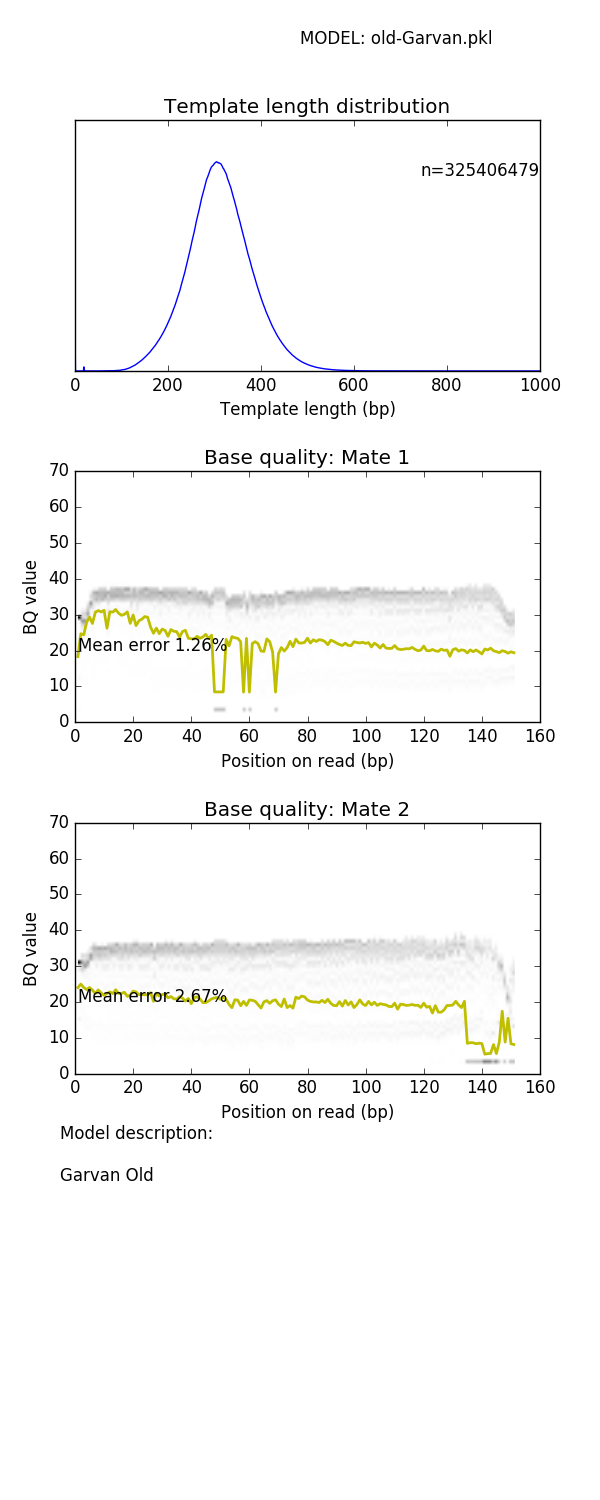
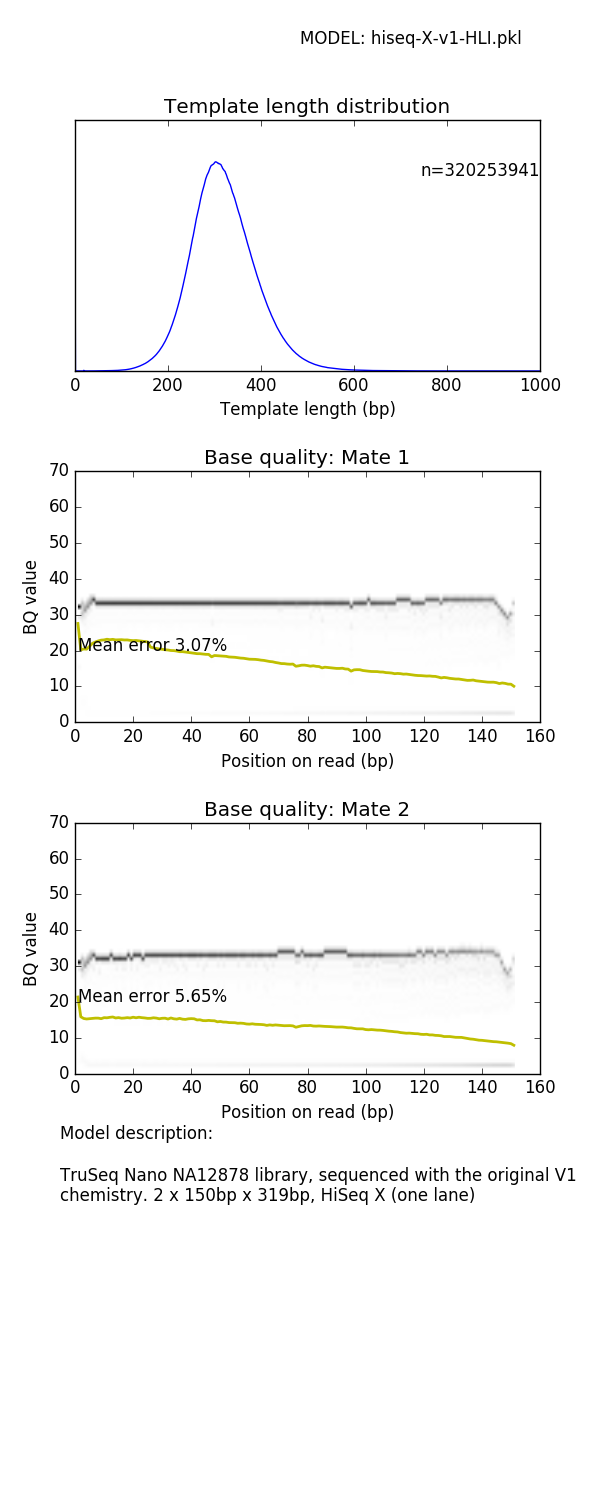
Built-in read models