Pixyz: A library for developing deep generative models


What is Pixyz?
Pixyz is a high-level deep generative modeling library, based on PyTorch. It is developed with a focus on enabling easy implementation of various deep generative models.
Recently, many papers about deep generative models have been published. However, its reproduction becomes a hard task, for both specialists and practitioners, because such recent models become more complex and there are no unified tools that bridge mathematical formulation of them and implementation. The vision of our library is to enable both specialists and practitioners to implement such complex deep generative models by just as if writing the formulas provided in these papers.
Our library supports the following deep generative models.
- Explicit models (likelihood-based)
- Variational autoencoders (variational inference)
- Flow-based models
- Autoregressive generative models (note: not implemented yet)
- Implicit models
- Generative adversarial networks
Moreover, Pixyz enables you to implement these different models in the same framework and in combination with each other.
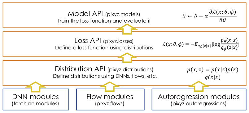
The overview of Pixyz is as follows. Each API will be discussed below.
Note: Since this library is under development, there are possibilities to have some bugs.
Installation
Pixyz can be installed by using pip.
$ pip install pixyz
If installing from source code, execute the following commands.
$ git clone https://github.com/masa-su/pixyz.git
$ pip install -e pixyz
You can also install pixyz and PyTorch environment through Docker Hub
# pull docker image from https://hub.docker.com/r/kenoharada/pixyz
$ docker pull kenoharada/pixyz:v0.3.0_python_3.7.7_pytorch_1.6.0_cuda_10.1

# Run pixyz environment
$ docker run --runtime=nvidia -e NVIDIA_VISIBLE_DEVICES=0 --rm -it kenoharada/pixyz:v0.3.0_python_3.7.7_pytorch_1.6.0_cuda_10.1
Quick Start
Here, we consider to implement a variational auto-encoder (VAE) which is one of the most well-known deep generative models. VAE is composed of a inference model
and a generative model
, each of which is defined by DNN, and this loss function (negative ELBO) is as follows.
(1)
In Pixyz, deep generative models are implemented in the following three steps:
- Define distributions(Distribution API)
- Set the loss function of a model(Loss API)
- Train the model(Model API)
1. Define distributions(Distribution API)
First, we need to define two distributions (
,
) with DNNs. In Pixyz, you can do this by building DNN modules just as you do in PyTorch. The main difference is that you should inherit the
pixyz.distributions.* class (Distribution API), instead of torch.nn.Module .
For example,
(Bernoulli)
and
(normal) are implemented as follows.
>>> from pixyz.distributions import Bernoulli, Normal
>>> # inference model (encoder) q(z|x)
>>> class Inference(Normal):
...     def __init__(self):
...         super(Inference, self).__init__(var=["z"],cond_var=["x"],name="q")  # var: variables of this distribution, cond_var: coditional variables.
...         self.fc1 = nn.Linear(784, 512)
...         self.fc21 = nn.Linear(512, 64)
...         self.fc22 = nn.Linear(512, 64)
...
...     def forward(self, x):  # the name of this argument should be same as cond_var.
...         h = F.relu(self.fc1(x))
...         return {"loc": self.fc21(h),
...                 "scale": F.softplus(self.fc22(h))}  # return parameters of the normal distribution
...
>>> # generative model (decoder) p(x|z)
>>> class Generator(Bernoulli):
...     def __init__(self):
...         super(Generator, self).__init__(var=["x"], cond_var=["z"], name="p")
...         self.fc1 = nn.Linear(64, 512)
...         self.fc2 = nn.Linear(512, 128)
...
...     def forward(self, z):  # the name of this argument should be same as cond_var.
...         h = F.relu(self.fc1(z))
...         return {"probs": F.sigmoid(self.fc2(h))}    # return a parameter of the Bernoulli distribution
Once defined, you can create instances of these classes.
>>> p = Generator()
>>> q = Inference()
In VAE,
, a prior of the generative model, is usually defined as the standard normal distribution, without using DNNs.
Such an instance can be created from
pixyz.distributions.* as
>>> prior = Normal(loc=torch.tensor(0.), scale=torch.tensor(1.),
...                var=["z"], features_shape=[64], name="p_prior")
If you want to find out what kind of distribution each instance defines and what modules (the network architecture) define it, just print them.
>>> print(p)
Distribution:
  p(x|z)
Network architecture:
  Generator(
    name=p, distribution_name=Bernoulli,
    var=['x'], cond_var=['z'], input_var=['z'], features_shape=torch.Size([])
    (fc1): Linear(in_features=64, out_features=512, bias=True)
    (fc2): Linear(in_features=512, out_features=512, bias=True)
    (fc3): Linear(in_features=512, out_features=784, bias=True)
  )
If you are working on the iPython environment, you can use print_latex to display them in the LaTeX compiled format.

Conveniently, each distribution instance can perform sampling over given samples, regardless of the form of the internal DNN modules.
>>> samples_z = prior.sample(batch_n=1)
>>> print(samples_z)
{'z': tensor([[ 0.6084,  1.4716,  0.6413,  1.3184, -0.8930,  0.0603,  1.2254,  0.5910, ..., 0.8389]])}
>>> samples = p.sample(samples_z)
>>> print(samples)
{'z': tensor([[ 1.5377,  0.4713,  0.0354,  0.5013,  1.2584,  0.8908,  0.6323,  1.0844, ..., -0.7603]]),
 'x': tensor([[0., 1., 0., 1., 0., 0., 1., 1., 0., 0., 1., 1., 1., 1., ..., 0.]])}
As in this example, samples are represented in dictionary forms in which the keys correspond to random variable names and the values are their realized values.
Moreover, the instance of joint distribution
can be created by the product of distribution instances.
>>> p_joint = p * priorThis instance can be checked as
>>> print(p_joint)
Distribution:
  p(x,z) = p(x|z)p_{prior}(z)
Network architecture:
  Normal(
    name=p_{prior}, distribution_name=Normal,
    var=['z'], cond_var=[], input_var=[], features_shape=torch.Size([64])
    (loc): torch.Size([1, 64])
    (scale): torch.Size([1, 64])
  )
  Generator(
    name=p, distribution_name=Bernoulli,
    var=['x'], cond_var=['z'], input_var=['z'], features_shape=torch.Size([])
    (fc1): Linear(in_features=64, out_features=512, bias=True)
    (fc2): Linear(in_features=512, out_features=512, bias=True)
    (fc3): Linear(in_features=512, out_features=784, bias=True)
  )
Also, it can perform sampling in the same way.
>>> p_joint.sample(batch_n=1)
{'z': tensor([[ 1.5377,  0.4713,  0.0354,  0.5013,  1.2584,  0.8908,  0.6323,  1.0844, ..., -0.7603]]),
 'x': tensor([[0., 1., 0., 1., 0., 0., 1., 1., 0., 0., 1., 1., 1., 1., ..., 0.]])}
By constructing the joint distribution in this way, you can easily implement more complicated generative models.
2. Set the loss function of a model(Loss API)
Next, we set the objective (loss) function of the model with defined distributions.
Loss API (pixyz.losses.*) enables you to define such loss function as if just writing mathematic formulas. The loss function of VAE (Eq.(1)) can easily be converted to the code style as follows.
>>> from pixyz.losses import KullbackLeibler, LogProb, Expectation as E
>>> reconst = -E(q, LogProb(p)) # the reconstruction loss (it can also be written as `-p.log_prob().expectation()`)
>>> kl = KullbackLeibler(q,prior) # Kullback-Leibler divergence
>>> loss_cls = (kl + reconst).mean()
Like Distribution API, you can check the formula of the loss function by printing.
>>> print(loss_cls)
mean \left(D_{KL} \left[q(z|x)||p_{prior}(z) \right] - \mathbb{E}_{q(z|x)} \left[\log p(x|z) \right] \right) 
When evaluating this loss function given data, use the eval method.
>>> loss_tensor = loss_cls.eval({"x": x_tensor}) # x_tensor: input data
>>> print(loss_tensor)
tensor(1.00000e+05 * 1.2587)
3. Train the model(Model API)
Finally, Model API (pixyz.models.Model) can train the loss function given the optimizer, distributions to train, and training data.
>>> from pixyz.models import Model
>>> from torch import optim
>>> model = Model(loss_cls, distributions=[p, q],
...               optimizer=optim.Adam, optimizer_params={"lr":1e-3}) # initialize a model
>>> train_loss = model.train({"x": x_tensor}) # train the model given training data (x_tensor)
After training the model, you can perform generation and inference on the model by sampling from
and
, respectively.
More information
These frameworks of Pixyz allow the implementation of more complex deep generative models. See sample codes and the pixyzoo repository as examples.
For more detailed usage, please check the Pixyz documentation.
If you encounter some problems in using Pixyz, please let us know.
Citation
@misc{suzuki2021pixyz,
      title={Pixyz: a library for developing deep generative models},
      author={Masahiro Suzuki and Takaaki Kaneko and Yutaka Matsuo},
      year={2021},
      eprint={2107.13109},
      archivePrefix={arXiv},
      primaryClass={cs.LG}
}
Acknowledgements
This library is based on results obtained from a project commissioned by the New Energy and Industrial Technology Development Organization (NEDO).


