Psitip

Python Symbolic Information Theoretic Inequality Prover

Psitip is a computer algebra system for information theory written in Python. Random variables, expressions and regions are objects in Python that can be manipulated easily. Moreover, it implements a versatile deduction system for automated theorem proving. Psitip supports features such as:

• Proving linear information inequalities via the linear programming method by Yeung and Zhang (see References). The linear programming method was first implemented in the ITIP software developed by Yeung and Yan ( http://user-www.ie.cuhk.edu.hk/~ITIP/ ). See References for other software based on this method.
• Proving first-order logic statements on random variables (involving arbitrary combinations of information inequalities, existence, uniqueness, and, or, not, implication, etc).
• Automated inner and outer bounds for multiuser settings in network information theory (see the Jupyter Notebook examples ).
• Numerical optimization over distributions, and evaluation of rate regions involving auxiliary random variables (e.g. Example 1: Degraded broadcast channel).
• Interactive mode and Parsing LaTeX code.
• Finding examples of distributions where a set of constraints is satisfied.
• Fourier-Motzkin elimination.
• Discover inequalities via the convex hull method for polyhedron projection [Lassez-Lassez 1991].
• Non-Shannon-type inequalities.
• Integration with Jupyter Notebook and LaTeX output.
• Generation of Human-readable Proof.
• Drawing Information diagrams.
• User-defined information quantities (see Real-valued information quantities, e.g. information bottleneck, and Wyner's CI and Gács-Körner CI in the example below).
• Bayesian network optimization. Psitip is optimized for random variables following a Bayesian network structure, which can greatly improve performance.

Examples with Jupyter Notebook (ipynb file) :

from psitip import *
PsiOpts.setting(solver = "pyomo.glpk")     # Set linear programming solver
PsiOpts.setting(repr_latex = True)         # Jupyter Notebook LaTeX display
PsiOpts.setting(venn_latex = True)         # LaTeX in diagrams
PsiOpts.setting(proof_note_color = "blue") # Reasons in proofs are blue

X, Y, Z, W, U, M, S = rv("X, Y, Z, W, U, M, S") # Declare random variables

H(X+Y) - H(X) - H(Y)  # Simplify H(X,Y) - H(X) - H(Y)

bool(H(X) + I(Y & Z | X) >= I(Y & Z))  # Check H(X) + I(Y;Z|X) >= I(Y;Z)

True

(markov(X+W, Y, Z) >> (I(X & W | Y) / 2 <= H(X | Z))).display_bool() # Implication

# Proof of the implication
(markov(X+W, Y, Z) >> (I(X & W | Y) / 2 <= H(X | Z))).proof(detail = True)

# Information diagram that shows the above implication
(markov(X+W, Y, Z) >> (I(X & W | Y) / 2 <= H(X | Z))).venn()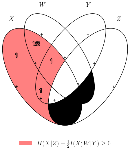

<Figure size 432x288 with 0 Axes>

# The condition "X is independent of Y and X-Y-Z forms a
# Markov chain" can be simplified to "X is independent of (Y,Z)"
markov(X, Y, Z) & indep(X, Y)

# The condition "there exists Y independent of X such that
# X-Y-Z forms a Markov chain" can be simplified to "X,Z independent"
(markov(X, Y, Z) & indep(X, Y)).exists(Y).simplified()

User-defined information quantities

# Define Gács-Körner common information [Gács-Körner 1973]
gkci = ((H(U|X) == 0) & (H(U|Y) == 0)).maximum(H(U), U)

# Define Wyner's common information [Wyner 1975]
wci = markov(X, U, Y).minimum(I(U & X+Y), U)

# Define common entropy [Kumar-Li-El Gamal 2014]
eci = markov(X, U, Y).minimum(H(U), U)

(gkci <= I(X & Y)).display_bool()        # Gács-Körner <= I(X;Y)

(I(X & Y) <= wci).display_bool()         # I(X;Y) <= Wyner

(wci <= emin(H(X), H(Y))).display_bool() # Wyner <= min(H(X),H(Y))

(gkci <= wci).proof(detail = True) # Output proof of Gács-Körner <= Wyner

# Automatically discover inequalities among quantities
universe().discover([X, Y, gkci, wci, eci])

# The meet or Gács-Körner common part [Gács-Körner 1973] between X and Y
# is a function of the GK common part between X and (Y,Z)
(H(meet(X, Y) | meet(X, Y + Z)) == 0).display_bool()

Automatic inner/outer bound for degraded broadcast channel

X, Y, Z = rv("X, Y, Z")
M1, M2 = rv_array("M", 1, 3)
R1, R2 = real_array("R", 1, 3)

model = CodingModel()
model.add_node(M1+M2, X)  # Encoder maps M1,M2 to X
model.add_edge(X, Y)      # Channel X -> Y -> Z
model.add_edge(Y, Z)
model.add_node(Y, M1)     # Decoder1 maps Y to M1
model.add_node(Z, M2)     # Decoder2 maps Z to M2
model.set_rate(M1, R1)    # Rate of M1 is R1
model.set_rate(M2, R2)    # Rate of M2 is R2

model.graph()             # Draw diagram

# Inner bound via [Lee-Chung 2015], give superposition region [Bergmans 1973], [Gallager 1974]
r = model.get_inner()
r

r_out = model.get_outer() # Automatic outer bound

# Converse proof, print auxiliary random variables
(r_out >> r).check_getaux_array()

# Output the converse proof
(model.get_outer(is_proof = True) >> r).proof()

r.maximum(R1 + R2, [R1, R2])          # Max sum rate

r.maximum(emin(R1, R2), [R1, R2])     # Max symmetric rate

r.exists(R1)   # Eliminate R1, same as r.projected(R2)

# Eliminate Z, i.e., taking union of the region over all choices of Z
# The program correctly deduces that it suffices to consider Z = Y
r.exists(Z).simplified()

Non-Shannon-type Inequalities

# Zhang-Yeung inequality [Zhang-Yeung 1998] cannot be proved by Shannon-type inequalities
(2*I(Z&W) <= I(X&Y) + I(X & Z+W) + 3*I(Z&W | X) + I(Z&W | Y)).display_bool()

# Using copy lemma [Zhang-Yeung 1998], [Dougherty-Freiling-Zeger 2011]
# You may use the built-in "with copylem().assumed():" instead of the below
with eqdist([X, Y, U], [X, Y, Z]).exists(U).forall(X+Y+Z).assumed():

    # Prove Zhang-Yeung inequality
    (2*I(Z&W) <= I(X&Y) + I(X & Z+W) + 3*I(Z&W | X) + I(Z&W | Y)).display_bool()

# State the copy lemma
r = eqdist([X, Y, U], [X, Y, Z]).exists(U)

# Automatically discover non-Shannon-type inequalities using copy lemma
PsiOpts.setting(discover_max_facet = None) # Unlimited number of facets
r.discover([X, Y, Z, W]).simplified()

About

Author: Cheuk Ting Li ( https://www.ie.cuhk.edu.hk/people/ctli.shtml ). The source code of Psitip is released under the GNU General Public License v3.0 ( https://www.gnu.org/licenses/gpl-3.0.html ). The author would like to thank Raymond W. Yeung and Chandra Nair for their invaluable comments.

The working principle of Psitip (existential information inequalities) is described in the following article:

• C. T. Li, "An Automated Theorem Proving Framework for Information-Theoretic Results," arXiv preprint, available: https://arxiv.org/pdf/2101.12370.pdf , 2021.

If you find Psitip useful in your research, please consider citing the above article.

WARNING

This program comes with ABSOLUTELY NO WARRANTY. This program is a work in progress, and bugs are likely to exist. The deduction system is incomplete, meaning that it may fail to prove true statements (as expected in most automated deduction programs). On the other hand, declaring false statements to be true should be less common. If you encounter a false accept in Psitip, please let the author know.

Installation

Download psitip.py and place it in the same directory as your code, or open an IPython shell in the same directory as psitip.py. The file test.py and the Jupyter Notebook examples contain examples of usages of Psitip. Use from psitip import * in your code to import all functions in psitip.

Python 3 and numpy are required to run psitip. It also requires at least one of the following for sparse linear programming:

• Pyomo (https://github.com/Pyomo/pyomo). Recommended. Requires GLPK (installed separately) or another solver.
• PuLP (https://github.com/coin-or/pulp). Can use GLPK (installed separately), CBC (https://github.com/coin-or/Cbc , provided with PuLP, not recommended) or another solver.
• GLPK (https://www.gnu.org/software/glpk/). Recommended. An external solver to be used with PuLP or Pyomo. Can be installed using Conda (see https://anaconda.org/conda-forge/glpk ).
• SciPy (https://www.scipy.org/). Not recommended for problems with more than 8 random variables.

See the Solver section for details.

Other optional dependencies:

• Pycddlib (https://github.com/mcmtroffaes/pycddlib/), a Python wrapper for Komei Fukuda's cddlib (https://people.inf.ethz.ch/fukudak/cdd_home/). Needed only for the convex hull method for polyhedron projection (Discover inequalities).
• PyTorch (https://pytorch.org/). Needed only for Numerical optimization over probability distributions.
• Matplotlib (https://matplotlib.org/). Required for drawing Information diagrams.
• Graphviz (https://graphviz.org/). A Python binding of Graphviz is required for drawing Bayesian networks and communication network model.
• Lark (https://github.com/lark-parser/lark). A parsing toolkit. Required for Interactive mode and Parsing LaTeX code.

Solver

The default solver is Scipy, though it is highly recommended to switch to another solver, e.g.:

from psitip import *
PsiOpts.setting(solver = "pulp.glpk")
PsiOpts.setting(solver = "pyomo.glpk")
PsiOpts.setting(solver = "pulp.cbc") # Not recommended

PuLP supports a wide range of solvers (see https://coin-or.github.io/pulp/technical/solvers.html ). Use the following line to set the solver to any supported solver (replace ??? with the desired solver):

PsiOpts.setting(solver = "pulp.???")
PsiOpts.setting(pulp_solver = pulp.solvers.GLPK(msg = 0)) # If the above does not work

For Pyomo (see https://pyomo.readthedocs.io/en/stable/solving_pyomo_models.html#supported-solvers ), use the following line (replace ??? with the desired solver):

PsiOpts.setting(solver = "pyomo.???")

See Options for options for the solver.

WARNING: It is possible for inaccuracies in the solver to result in wrong output in Psitip. Try switching to another solver if a problem is encountered.

Basics

The following classes and functions are in the psitip module. Use from psitip import * to avoid having to type psitip.something every time you use one of these functions.

• Random variables are declared as X = rv("X"). The name "X" passed to "rv" must be unique. Variables with the same name are treated as being the same. The return value is a Comp object (compound random variable).

• As a shorthand, you may declare multiple random variables in the same line as X, Y = rv("X, Y"). Variable names are separated by ", " (the space cannot be omitted).

• The joint random variable (X,Y) is expressed as X + Y (a Comp object).
• Entropy H(X) is expressed as H(X). Conditional entropy H(X|Y) is expressed as H(X | Y). Conditional mutual information I(X;Y|Z) is expressed as I(X & Y | Z). The return values are Expr objects (expressions).
• Real variables are declared as a = real("a"). The return value is an Expr object (expression).
• Expressions can be added and subtracted with each other, and multiplied and divided by scalars, e.g. I(X + Y & Z) * 3 - a * 4.

• While Psitip can handle affine expressions like H(X) + 1 (i.e., adding or subtracting a constant), affine expressions are unrecommended as they are prone to numerical error in the solver.
• While expressions can be multiplied and divided by each other (e.g. H(X) * H(Y)), most symbolic capabilities are limited to linear and affine expressions. Numerical only: non-affine expressions can be used in concrete models, and support automated gradient for numerical optimization tasks, but do not support most symbolic capabilities for automated deduction.
• We can take power (e.g. H(X) ** H(Y)) and logarithm (using the elog function, e.g. elog(H(X) + H(Y))) of expressions. Numerical only: non-affine expressions can be used in concrete models, and support automated gradient for numerical optimization tasks, but do not support most symbolic capabilities for automated deduction.

• When two expressions are compared (using <=, >= or ==), the return value is a Region object (not a bool). The Region object represents the set of distributions where the condition is satisfied. E.g. I(X & Y) == 0, H(X | Y) <= H(Z) + a.

• While Psitip can handle general affine and half-space constraints like H(X) <= 1 (i.e., comparing an expression with a nonzero constant, or comparing affine expressions), they are unrecommended as they are prone to numerical error in the solver.
• While Psitip can handle strict inequalities like H(X) > H(Y), strict inequalities are unrecommended as they are prone to numerical error in the solver.

• The intersection of two regions (i.e., the region where the conditions in both regions are satisfied) can be obtained using the "&" operator. E.g. (I(X & Y) == 0) & (H(X | Y) <= H(Z) + a).

• To build complicated regions, it is often convenient to declare r = universe() (universe() is the region without constraints), and add constraints to r by, e.g., r &= I(X & Y) == 0.

• The union of two regions can be obtained using the "|" operator. E.g. (I(X & Y) == 0) | (H(X | Y) <= H(Z) + a). (Note that the return value is a RegionOp object, a subclass of Region.)
• The complement of a region can be obtained using the "~" operator. E.g. ~(H(X | Y) <= H(Z) + a). (Note that the return value is a RegionOp object, a subclass of Region.)
• The Minkowski sum of two regions (with respect to their real variables) can be obtained using the "+" operator.
• A region object can be converted to bool, returning whether the conditions in the region can be proved to be true (using Shannon-type inequalities). E.g. bool(H(X) >= I(X & Y)).
• The constraint that X, Y, Z are mutually independent is expressed as indep(X, Y, Z) (a Region object). The function indep can take any number of arguments.

• The constraint that X, Y, Z are mutually conditionally independent given W is expressed as indep(X, Y, Z).conditioned(W).

• The constraint that X, Y, Z forms a Markov chain is expressed as markov(X, Y, Z) (a Region object). The function markov can take any number of arguments.
• The constraint that X, Y, Z are informationally equivalent (i.e., contain the same information) is expressed as equiv(X, Y, Z) (a Region object). The function equiv can take any number of arguments. Note that equiv(X, Y) is the same as (H(X|Y) == 0) & (H(Y|X) == 0).
• The rv_seq method constructs a sequence of random variables. For example, X = rv_seq("X", 10) gives a Comp object consisting of X0, X1, ..., X9.

• A sequence can be used by itself to represent the joint random variable of the variables in the sequence. For example, H(X) gives H(X0,...,X9).
• A sequence can be indexed using X[i] (returns a Comp object). The slice notation in Python also works, e.g., X[5:-1] gives X5,X6,X7,X8 (a Comp object).
• The region where the random variables in the sequence are mutually independent can be given by indep(*X). The region where the random variables form a Markov chain can be given by markov(*X).

• Simplification Expr and Region objects have a simplify() method, which simplifies the expression/region in place. The simplified() method returns the simplified expression/region without modifying the object. For example, (H(X+Y) - H(X) - H(Y)).simplified() gives -I(Y & X).

• Note that calling Region.simplify() can take some time for the detection of redundant constraints. Use Region.simplify_quick() instead to skip this step.
• Use r.simplify(level = ???) to specify the simplification level (integer in 0,...,10). A higher level takes more time. The context manager PsiOpts.setting(simplify_level = ???): has the same effect.
• The simplify method always tries to convert the region to an equivalent form which is weaker a priori (e.g. removing redundant constraints and converting equality constraints to inequalities if possible). If a stronger form is desired, use r.simplify(strengthen = True).

• Logical implication. To test whether the conditions in region r1 imply the conditions in region r2 (i.e., whether r1 is a subset of r2), use r1.implies(r2) (which returns bool). E.g. (I(X & Y) == 0).implies(H(X + Y) == H(X) + H(Y)).

• Use r1.implies(r2, aux_hull = True) to allow rate splitting for auxiliary random variables, which may help proving the implication. This takes considerable computation time.
• Use r1.implies(r2, level = ???) to specify the simplification level (integer in 0,...,10), which may help proving the implication. A higher level takes more time.

• Logical equivalence. To test whether the region r1 is equivalent to the region r2, use r1.equiv(r2) (which returns bool). This uses implies internally, and the same options can be used.
• Use str(x) to convert x (a Comp, Expr or Region object) to string. The tostring method of Comp, Expr and Region provides more options. For example, r.tostring(tosort = True, lhsvar = R) converts the region r to string, sorting all terms and constraints, and putting the real variable R to the left hand side of all expressions (and the rest to the right).

Advanced

• Existential quantification is represented by the exists method of Region (which returns a Region). For example, the condition "there exists auxiliary random variable U such that R <= I(U;Y) - I(U;S) and U-(X,S)-Y forms a Markov chain" (as in Gelfand-Pinsker theorem) is represented by:

  ((R <= I(U & Y) - I(U & S)) & markov(U, X+S, Y)).exists(U)

• Calling exists on real variables will cause the variable to be eliminated by Fourier-Motzkin elimination. Currently, calling exists on real variables for a region obtained from material implication is not supported.
• Calling exists on random variables will cause the variable to be marked as auxiliary (dummy).
• Calling exists on random variables with the option toreal = True will cause all information quantities about the random variables to be treated as real variables, and eliminated using Fourier-Motzkin elimination. Those random variables will be absent in the resultant region (not even as auxiliary random variables). E.g.:

(indep(X+Z, Y) & markov(X, Y, Z)).exists(Y, toreal = True)

gives { I(Z;X) == 0 }. Note that using toreal = True can be extremely slow if the number of random variables is more than 5, and may cause false accepts (i.e., declaring a false inequality to be true) since only Shannon-type inequalities are enforced.

• Material implication between Region is denoted by the operator >>, which returns a Region object. The region r1 >> r2 represents the condition that r2 is true whenever r1 is true. Note that r1 >> r2 is equivalent to ~r1 | r2, and r1.implies(r2) is equivalent to bool(r1 >> r2).

• Material equivalence is denoted by the operator ==, which returns a Region object. The region r1 == r2 represents the condition that r2 is true if and only if r1 is true.

• Universal quantification is represented by the forall method of Region (which returns a Region). This is usually called after the implication operator >>. For example, the condition "for all U such that U-X-(Y1,Y2) forms a Markov chain, we have I(U;Y1) >= I(U;Y2)" (less noisy broadcast channel [Körner-Marton 1975]) is represented by:

  (markov(U,X,Y1+Y2) >> (I(U & Y1) >= I(U & Y2))).forall(U)

• Calling forall on real variables is supported, e.g. (((R == H(X)) | (R == H(Y))) >> (R == H(Z))).forall(R) gives (H(X) == H(Z)) & (H(Y) == H(Z)).
• Ordering of forall and exists among random variables are respected, i.e., r.exists(X1).forall(X2) is different from r.forall(X2).exists(X1). Ordering of forall and exists among real variables are also respected. Nevertheless, ordering between random variables and real variables are not respected, and real variables are always processed first (e.g., it is impossible to have (H(X) - H(Y) == R).exists(X+Y).forall(R), since it will be interpreted as (H(X) - H(Y) == R).forall(R).exists(X+Y)).

• Uniqueness is represented by the unique method of Region (which returns a Region). For example, to check that if X, Y are perfectly resolvable [Prabhakaran-Prabhakaran 2014], then their common part is unique:

  print(bool(((H(U | X)==0) & (H(U | Y)==0) & markov(X, U, Y)).unique(U)))

• Uniqueness does not imply existence. For both existence and uniqueness, use Region.exists_unique.

• Substitution. The function call r.substituted(x, y) (where r is an Expr or Region, and x, y are either both Comp or both Expr) returns an expression/region where all appearances of x in r are replaced by y. To replace x1 by y1, and x2 by y2, use r.substituted({x1: y1, x2: y2}) or r.substituted(x1 = y1, x2 = y2) (the latter only works if x1 has name "x1").

• Call substituted_aux instead of substituted to stop treating x as an auxiliary in the region r (useful in substituting a known value of an auxiliary).

• Minimization / maximization over an expression expr over variables v (Comp, Expr, or list of Comp and/or Expr) subject to the constraints in region r is represented by the r.minimum(expr, v) / r.maximum(expr, v) respectively (which returns an Expr object). For example, Wyner's common information [Wyner 1975] is represented by:

  markov(X, U, Y).minimum(I(U & X+Y), U)

• It is simple to define new information quantities. For example, to define the information bottleneck [Tishby-Pereira-Bialek 1999]:

  def info_bot(X, Y, t):
      U = rv("U")
      return (markov(U, X, Y) & (I(X & U) <= t)).maximum(I(Y & U), U)
  
  X, Y = rv("X, Y")
  t1, t2 = real("t1, t2")
  
  # Check that info bottleneck is non-decreasing
  print(bool((t1 <= t2) >> (info_bot(X, Y, t1) <= info_bot(X, Y, t2)))) # True
  
  # Check that info bottleneck is a concave function of t
  print(info_bot(X, Y, t1).isconcave()) # True
  
  # It is not convex in t
  print(info_bot(X, Y, t1).isconvex()) # False

• The minimum / maximum of two (or more) Expr objects is represented by the emin / emax function respectively. For example, bool(emin(H(X), H(Y)) >= I(X & Y)) returns True.

• The absolute value of an Expr object is represented by the abs function. For example, bool(abs(H(X) - H(Y)) <= H(X) + H(Y)) returns True.

• The projection of a Region r onto the real variable a is given by r.projected(a). All real variables in r other than a will be eliminated. For projection along the diagonal a + b, use r.projected(c == a + b) (where a, b, c are all real variables, and c is a new real variable not in r). To project onto multiple coordinates, use r.projected([a, b]) (where a, b are Expr objects for real variables, or Region objects for linear combinations of real variables). For example:

  # Multiple access channel capacity region without time sharing [Ahlswede 1971]
  r = indep(X, Y) & (R1 <= I(X & Z | Y)) & (R2 <= I(Y & Z | X)) & (R1 + R2 <= I(X+Y & Z))
  
  print(r.projected(R1))
  # Gives ( ( R1 <= I(X&Z+Y) ) & ( I(X&Y) == 0 ) )
  
  print(r.projected(R == R1 + R2)) # Project onto diagonal to get sum rate
  # Gives ( ( R <= I(X+Y&Z) ) & ( I(X&Y) == 0 ) )

  See Fourier-Motzkin elimination for another example. For a projection operation that also eliminates random variables, see Discover inequalities.

• While one can check the conditions in r (a Region object) by calling bool(r), to also obtain the auxiliary random variables, instead call r.check_getaux(), which returns a list of pairs of Comp objects that gives the auxiliary random variable assignments (returns None if bool(r) is False). For example:

  (markov(X, U, Y).exists(U).minimum(I(U & X+Y)) <= H(X)).check_getaux()

  returns [(U, X)].

• If branching is required (e.g. for union of regions), check_getaux may give a list of lists of pairs, where each list represents a branch. For example:

(markov(X, U, Y).exists(U).minimum(I(U & X+Y))
    <= emin(H(X),H(Y))).check_getaux()

returns [[(U, X)], [(U, X+Y)], [(U, Y)]].

• The function check_getaux_dict returns the results as a dict. The function check_getaux_array returns the results as a CompArray. These two methods should only be used on simple implications (without union, negation and maximization/minimization quantities).

• The meet or Gács-Körner common part [Gács-Körner 1973] between X and Y is denoted as meet(X, Y) (a Comp object).
• The minimal sufficient statistic of X about Y is denoted as mss(X, Y) (a Comp object).
• The random variable given by the strong functional representation lemma [Li-El Gamal 2018] applied on X, Y (Comp objects) with a gap term logg (Expr object) is denoted as sfrl_rv(X, Y, logg) (a Comp object). If the gap term is omitted, this will be the ordinary functional representation lemma [El Gamal-Kim 2011].
• To set a time limit to a block of code, start the block with with PsiOpts(timelimit = "1h30m10s100ms"): (e.g. for a time limit of 1 hour 30 minutes 10 seconds 100 milliseconds). This is useful for time-consuming tasks, e.g. simplification and optimization.
• Stopping signal file. To stop the execution of a block of code upon the creation of a file named "stop_file.txt", start the block with with PsiOpts(stop_file = "stop_file.txt"):. This is useful for functions with long and unpredictable running time (creating the file would stop the function and output the results computed so far).

Human-readable Proof

Calling r.proof() (where r is a Region) produces the step-by-step proof of the region r (the proof is a ProofObj object). Some options:

• r.proof(shorten = True) will shorten the proof by enforcing sparsity of dual variables via L1 regularization using a method similar to [Ho-Ling-Tan-Yeung 2020]. This can be quite slow. Default is True.

• If this is False, then a solver which supports outputting dual variables is required, e.g. PsiOpts.setting(solver = "pyomo.glpk").

• r.proof(step_bayesnet = True) will also output steps deduced using conditional independence in the Bayesian network. Setting to False makes the function considerably faster. Default is True.
• r.proof(step_chain = True) will display a chain of inequalities (instead of listing each step separately). Setting to False may make the proof more readable. Default is True.
• r.proof(step_optimize = True) will order the steps in the simplest manner. Setting to False makes the function considerably faster. Default is True.
• r.proof(note_skip_trivial = True) will skip reasons for trivial steps. Setting to False makes the function output reasons even for trivial steps. Default is True.
• r.proof(step_simplify = True) will display simplification steps. Default is False.
• r.proof(step_expand_def = True) will display steps for expanding definitions of user-defined information quantities. Default is False.
• r.proof(repeat_implicant = True) will display the implicant in an implication. Default is False.
• r.proof(note_newline = ???) will set the maximum length of a line until the reason is written on a separate line. Set to True/False to always/never write reasons in separate lines. This can also be set via the global setting PsiOpts.setting(proof_note_newline = ???).

• If breaking all long lines (not only the reasons) is desired, use PsiOpts.setting(latex_line_len = 80) to set the maximum line length of LaTeX output.

• r.proof(note_color = "blue") will display the reasons of each inequality in blue in LaTeX output (can accept any LaTeX color). This can also be set via the global setting PsiOpts.setting(proof_note_color = "blue").

A ProofObj object can be displayed via print(r.proof()) (plain text), print(r.proof().latex()) (LaTeX code), or r.proof().display() (LaTeX display in Jupyter Notebook).

To construct a longer proof consisting of several steps, start a block with with PsiOpts(proof_new = True):, and end it with print(PsiOpts.get_proof()) (to print the proof in plain text), print(PsiOpts.get_proof().latex()) (to print the proof in LaTeX) or PsiOpts.get_proof().display() (to typeset the proof in LaTeX and display in Jupyter Notebook). For example,

with PsiOpts(proof_new = True):
    bool(markov(X, Y, Z) >> (H(Y) >= I(X & Z)))
    print(PsiOpts.get_proof())

Also see Example 3: Lossy source coding with side information at decoder.

Interactive mode and Parsing LaTeX code

Interactive mode can be entered by calling the main function of the Psitip package (if the Psitip package is installed, type python -m psitip in the terminal). It has a lax syntax, accepting the Psitip syntax, common notations and LaTeX input. Common functions are check (checking the conditions), implies (material implication), simplify, assume (assume a region is true; assumption can be accessed via assumption, and cleared via clear assume) and latex (latex output). Parsing can also be accessed using Expr.parse("3I(X,Y;Z)") and Region.parse("3I(X,Y;Z) \le 2") in Python code (Jupyter Notebook example). Interactive mode examples:

> a = I(X ; Y Z)
I(X&Y+Z)

> check a = 0 implies exists U st H(U) = I(X ; Y | U) <= 0
True

> latex simplify \exists U : H(U | Y, Z) = 0, R \ge H(X | U)
R \ge H(X|Y, Z)

> assume X -> (Y,Z) -> W
markov(X, Y+Z, W)

> assumption
markov(X, Y+Z, W)

> check H(Y Z) >= I(X;W)
True

> I(X;W|Y,Z)
0

> clear assume

> assumption
universe()

Information diagrams

The venn method of Comp, Expr, Region and ConcModel draws the information diagram of that object. The venn method takes any number of arguments (Comp, Expr, Region or ConcModel) which are drawn together. For Region.venn, only the nonzero cells of the region will be drawn (the others are in black). The ordering of the random variables is decided by the first Comp argument (or automatically if no Comp argument is supplied). To draw a Karnaugh map instead of a Venn diagram, use table instead of venn. The methods venn and table take a style argument, which is a string with the following options (multiple options are separated by ","):

• blend: Blend the colors in overlapping areas. Default for venn.
• hatch: Use hatch instead of fill.
• pm: Use +/- instead of numbers.
• notext: Hide the numbers.
• nosign: Hide the signs of each cell (+/-) on the bottom of each cell.
• nolegend: Hide the legends.
• Add the line PsiOpts.setting(venn_latex = True) at the beginning to turn on LaTeX in the diagram.

Examples:

from psitip import *
X, Y, Z, W, U = rv("X", "Y", "Z", "W", "U")
(X+Y+Z).venn(H(X), H(Y) - H(Z))

(markov(X, Y, Z, W) & (H(W | Z) == 0)).venn(H(X), I(Y & W), style = "hatch,pm")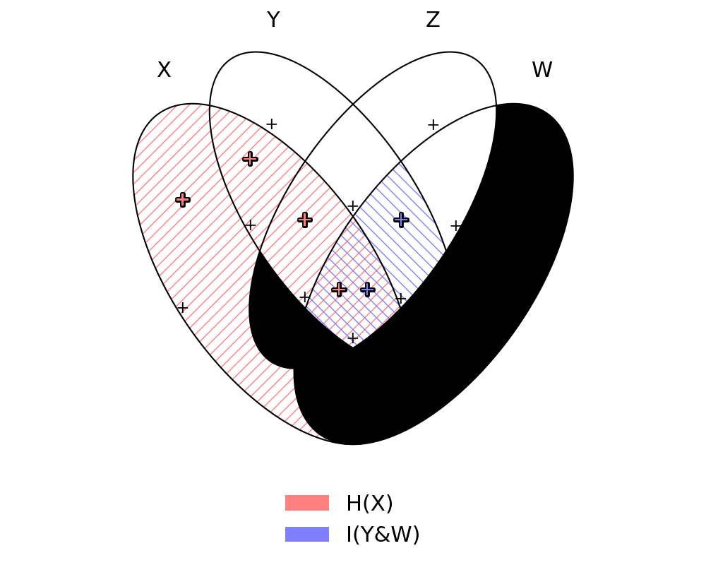

# Entropy, total correlation [Watanabe 1960] and dual total correlation [Han 1978]
# use Branko Grunbaum's Venn diagram for 5 variables
(X+Y+Z+W+U).venn(H(X+Y+Z+W+U), total_corr(X&Y&Z&W&U),
                dual_total_corr(X&Y&Z&W&U), style = "nolegend")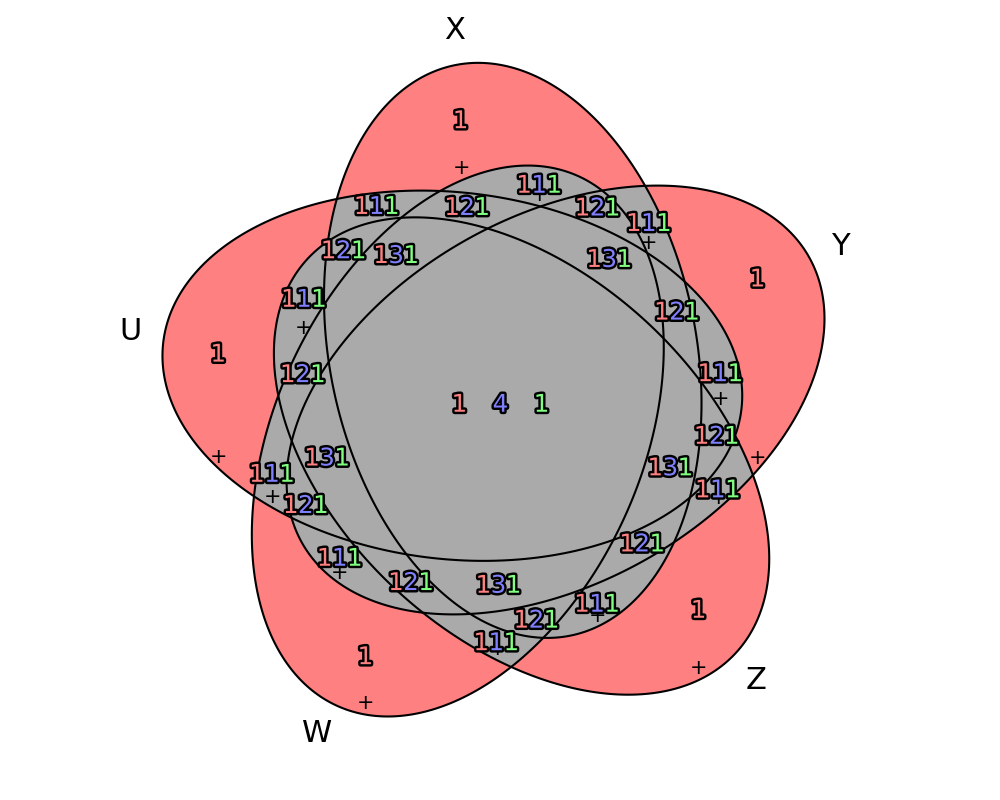

Numerical optimization

Psitip supports numerical optimization on distributions of random variables. While Comp are abstract random variables without information on their distributions, you can use a ConcModel object (concrete model) to assign joint distributions to random variables.

WARNING: Numerical optimization is prone to numerical errors. For nonconvex optimization, the algorithm is not guaranteed to find the global optimum.

Caution: In order to use the numerical functions of Psitip, the cardinality of random variables must be specified using set_card, e.g. X = rv("X").set_card(2). For numerical optimization, add the line PsiOpts.setting(istorch = True) at the beginning to enable PyTorch.

Concrete distributions

A (joint/conditional) distribution is stored as a ConcDist (concrete distribution) object. It is constructed as ConcDist(a, num_in), where a is the probability table (a numpy.array or torch.Tensor), and num_in is the number of random variables to be conditioned on. For example, if X -> Y is a Z-channel, P(Y|X) can be represented as ConcDist(array([[1.0, 0.0], [0.1, 0.9]]), num_in = 1). Note that for P(Y[0],...,Y[m-1] | X[0],...,X[n-1]), the number of dimensions of a is n+m, where the first n dimensions correspond to X[0],...,X[n-1], and the remaining m dimensions correspond to Y[0],...,Y[m-1].

• Some entries of the distribution can be Expr objects, e.g. we can have t = real("t"); p = ConcDist([1 - t, t]) for the distribution Bern(t). The distribution is automatically updated when the value of t changes. This is useful for optimizing over distributions parametrized by some parameters. See Example 4: Parametric distribution.
• If p is P(Y|X), and q is P(Z|X), then P(Y,Z|X) (assuming Y,Z are conditionally independent given X) is p * q.
• If p is P(Y|X), and q is P(Z|Y), then P(Z|X) is p @ q.
• If p is P(Y|X), and q is P(Z|Y), then P(Y,Z|X) is p.semidirect(q).
• If p is P(Y0,...,Y5|X), then P(Y2,Y4|X) is p.marginal(2,4).
• If p is P(Y|X), then P(Y|X=x) is p.given(x).
• If p is P(X), then E[f(X)] is p.mean(f). f is a function, numpy.array or torch.Tensor. If f is a function, the number of arguments must match the number of dimensions (random variables) of the joint distribution. If f is an array or tensor, shape must match the shape of the distribution.

• In both given and mean, the values of X are assumed to range from 0 to the cardinality of X minus 1. If X does not take these values, manual conversion is needed between the values of X and indices between 0 and the cardinality of X minus 1.

• p.numpy() gives the probability tensor as a numpy array. p.torch() gives the probability tensor as a PyTorch tensor.

Concrete model

Letting P = ConcModel(), we have the following operations:

• P[X] for a random variable (Comp) X gives the distribution of X (ConcDist). Use P[X] = p to set the distribution of X (where p is ConcDist, numpy.array or torch.Tensor). Use P[X+Y | Z+W] for the conditional distribution P(X,Y|Z,W).

• Some entries of the distribution can be Expr objects, e.g. we can have t = real("t"); P[X] = [1 - t, t] to represent X ~ Bern(t). The distribution is automatically updated when the value of t changes. This is useful for optimizing over distributions parametrized by some parameters. See Example 4: Parametric distribution.
• Random variables must be added to the model in the order they are generated. E.g., P[X] = p1; P[Y|X] = p2; P[Z|Y] = p3. If Z is added as P[Z|Y] = p3, it is assumed to be conditionally independent of all previously added random variables given Y.
• P[Y|X] = "var" specifys that P(Y|X) is a variable that can be optimized over. Use P[Y|X] = "var,rand" to randomize its initial value (otherwise the initial value is uniform, which may not be desirable for some optimization tasks).
• P[X] = "unif" specifys that X is uniformly distributed over 0, ..., X.get_card()-1 (shorthand of P[X] = ConcDist.uniform(X.get_card())).
• P[Z|X+Y] = "add" specifys that Z = X + Y (the "+" here is addition between integers, not joint random variable).
• P[Z|X+Y] = "flat" specifys that Z = X * Y.get_card() + Y, i.e., Z is an integer in the range 0, ..., X.get_card()*Y.get_card()-1 which contains the same information as (X, Y).

• P[a] for an expression (Expr) a gives the value of a (as a ConcReal object) under the distribution in P. E.g. P[I(X & Y) - H(Z | Y)].

• Use float(P[I(X & Y)]) to convert the ConcReal to a float. Use P[I(X & Y)].torch() to convert the ConcReal to a PyTorch tensor.
• Note that P[a] is read-only except when a is a single real variable. In that case, P[a]=1.0 sets the value of the real variable to 1.0. Use P[a]=ConcReal(1.0, lbound = 0.0, ubound = 10.0, isvar = True) to set a to be a variable that can be optimized over, with lower bound lbound and upper bound ubound.
• Shorthand: P[a] = "var" specifys that a is a variable that can be optimized over.

• P[r] for a region (Region) r gives the truth value of the conditions in r.
• P.venn() draws the information diagram of the random variables.
• P.graph() gives the Bayesian network of the random variables as a Graphviz graph.

Useful functions

Letting X, Y, Z = rv("X", "Y", "Z"),

• X.prob(x) (an Expr object) gives the probability P(X=x). For joint probability, (X+Y).prob(x, y) gives P(X=x, Y=y).

• X.pmf() gives the whole probability vector (an ExprArray object). (X+Y+Z).pmf() gives the probability tensor of X,Y,Z. (X|Y).pmf() gives the transition matrix. ExprArray objects support basic numpy-array-like operations such as +, -, *, @, dot, transpose, trace, diag, reshape.
• Note that X.prob(x) gives an abstract expression (Expr). To evaluate it on a concrete model P, use P[X.prob(x)] as mentioned in the Concrete model section. This can also be used on ExprArray, e.g. P[X.pmf()] gives the same result as P[X].

• X.mean(f) (an Expr object) gives the expectation E[f(X)]. For joint probability, (X+Y).mean(f) gives E[f(X, Y)]. The parameter f follows the same requirements as ConcDist.mean above.
• For other functions e.g. divergence, Rényi entropy, maximal correlation, varentropy, see Real-valued information quantities and Real-valued information quantities (numerical only).
• For general user-defined functions, use Expr.fcn to wrap any function mapping a ConcModel to a number as an Expr. E.g. the Hamming distortion is given by Expr.fcn(lambda P: P[X+Y].mean(lambda x, y: float(x != y))). For optimization using PyTorch, the return value should be a scalar torch.Tensor with gradient information.

Optimization

The function ConcModel.minimize(expr, vs, reg) (or maximize) takes 3 arguments: expr (Expr object) is the optimization objective, vs (ConcDist, ConcReal, or a list of these objects) specifies the variables to be optimized over, and reg (Region object, optional) specifies the constraints. The return value is the minimum (or maximum).

• reg may contain auxiliary random variable s that are not already in the model. The auxiliary random variables are added to the model automatically.
• After calling P.minimize, the optimal distributions are written to P, and can be obtained via e.g. P[X+Y].

• Note that P only contains distributions of random variables originally in P before calling P.minimize. To also obtain the distributions of auxiliary random variables (e.g. U), use P.opt_model()[U].

• General functions (not only linear combinations of entropy) may be used in expr and reg using Expr.fcn (see Useful functions).
• Use PsiOpts.setting(opt_optimizer = ???) to choose the optimization method. The default algorithm is "SLSQP" via scipy.optimize [Kraft 1988], which is suitable for convex problems (e.g. channel capacity, rate-distortion). Other choices are "sgd" (gradient descent) and "adam" [Kingma 2014] via PyTorch.
• Use PsiOpts.setting(opt_basinhopping = True) to enable basin hopping [Wales-Doye 1997] for nonconvex problems (e.g. problems involving auxiliary random variables).

• Use PsiOpts.setting(opt_num_hop = 50) to set the number of hops for basin hopping.

• Use PsiOpts.setting(opt_num_iter = 100) to set the number of iterations. Use PsiOpts.setting(opt_num_iter_mul = 2) to multiply to the number of iterations.
• Use PsiOpts.setting(opt_num_points = 10) to set the number of random initial points to try.
• Use PsiOpts.setting(opt_aux_card = 3) to set the default cardinality of the auxiliary random variables where set_card has not been called.
• Use PsiOpts.setting(verbose_opt = True) and PsiOpts.setting(verbose_opt_step = True) to display steps.

• Finding examples. For a Region r, to find an example of distributions of random variables where r is satisfied, use r.example(), which returns a ConcModel. E.g. P = ((I(X & Y) == 0.2) & (H(X) == 0.3)).example(); print(P[X+Y]). It uses ConcModel.minimize internally, and all above options apply (turning on opt_basinhopping is highly recommended).

Example 1: Channel coding, finding optimal input distribution

# ********** Channel input distribution optimization **********

import numpy
import scipy
import torch
from psitip import *
PsiOpts.setting(solver = "pyomo.glpk")
PsiOpts.setting(istorch = True)     # Enable pytorch

X, Y = rv("X", "Y").set_card(2)     # X,Y are binary RVs (cardinality = 2)
P = ConcModel()                     # Underlying distribution of RVs
P[X] = [0.3, 0.7]                   # Distribution of X is Bernoulli(0.7)
P[Y | X] = [[0.8, 0.2], [0.2, 0.8]] # X->Y is BSC(0.2)

print(P[Y])                         # Print distribution of Y
print(P[I(X & Y)])                  # Print I(X;Y)

P[X] = "var"                        # P[X] is a variable in optimization
P.maximize(I(X & Y), P[X])          # Maximize I(X;Y) over variable P[X]

print(P[I(X & Y)])                  # Print optimal I(X;Y)
print(P[X])                         # Print distribution of X attaining optimum
P.venn()                            # Draw information diagram

Example 2: Lossy source coding, rate-distortion

# ********** Rate-distortion **********

import numpy
import scipy
import torch
from psitip import *
PsiOpts.setting(solver = "pyomo.glpk")
PsiOpts.setting(istorch = True) # Enable pytorch

X, Y = rv("X", "Y").set_card(2) # X,Y are binary RVs (cardinality = 2)
P = ConcModel()                 # Underlying distribution of RVs
P[X] = [0.3, 0.7]               # Distribution of X is Bernoulli(0.7)
P[Y | X] = "var"                # P[Y | X] is a variable in optimization

# Hamming distortion function is the mean of the function 1{x != y}
# over the distribution P(X,Y). We demonstrate 4 methods to specify it:
# Method 1: Use the mean function
dist = (X+Y).mean(lambda x, y: float(x != y))

# Method 2: Distortion = P(X=0,Y=1) + P(X=1,Y=0)
# dist = (X+Y).prob(0, 1) + (X+Y).prob(1, 0)

# Method 3: Use "pmf" to obtain probability matrix (ExprArray object)
# and take 1 - trace
# dist = 1 - (X+Y).pmf().trace()

# Method 4: Use Expr.fcn to wrap any function
# mapping a ConcModel to a number as an Expr
# dist = Expr.fcn(lambda P: P[X+Y][0, 1] + P[X+Y][1, 0])

# Minimize I(X;Y) over P[Y | X], under constraint dist <= 0.1
P.minimize(I(X & Y), P[Y | X], dist <= 0.1)

print(P[I(X & Y)])        # print optimal I(X;Y)
print(P[Y | X].given(0))  # print P[Y | X=0] attaining optimum
print(P[Y | X].given(1))  # print P[Y | X=1] attaining optimum
print(P[dist])            # print distortion
P.venn()                  # draw information diagram

Example 3: Finding the most informative bit

# ********** Finding the most informative bit **********
# Kumar and Courtade, "Which boolean functions are
# most informative?", ISIT 2013
# Given X1,...,Xn i.i.d. fair bits, and Y1,...,Yn produced by passing
# X1,...,Xn through a memoryless BSC, the problem is to find a binary
# function F(X1,...,Xn) that maximizes I(F;Y)

import numpy
import scipy
import torch
from psitip import *
PsiOpts.setting(solver = "pyomo.glpk")
PsiOpts.setting(istorch = True)       # Enable pytorch
# PsiOpts.setting(verbose_opt = True) # Uncomment to display steps
# PsiOpts.setting(verbose_opt_step = True)

n = 3
a = 0.1

X = rv_seq("X", n).set_card(2) # X,Y are array of bits (cardinality = 2)
Y = rv_seq("Y", n).set_card(2)
F = rv("F").set_card(2)        # F is a binary random variable
P = ConcModel()                # Underlying distribution of RVs

# Add random variables to the model in the order they are generated
for x, y in zip(X, Y):
    P[x] = ConcDist.bit()      # P(x) is Bernoulli(1/2)
    P[y | x] = ConcDist.bsc(a) # P(y|x) is BSC with crossover a

P[F | X] = "var,rand"          # P(F|X) is the variable we optimize over

# Maximize I(F ; Y1,Y2,Y3)
# The default setting is not suitable for nonconvex optimization
print(P.maximize(I(F & Y), P[F | X]))
print(P[F | X])
print(P[I(F & Y)])

# Switch to basin-hopping for nonconvex optimization
PsiOpts.setting(opt_basinhopping = True)
PsiOpts.setting(opt_num_iter_mul = 2) # double the number of iterations

# "timelimit = 60000" sets time limit 60000ms for code within the block
with PsiOpts(timelimit = 60000):
    print(P.maximize(I(F & Y), P[F | X]))
print(P[F | X])
print(P[I(F & Y)])

Example 4: Parametric distribution

# ********** Parametric distribution **********

import numpy
import scipy
import torch
from psitip import *
PsiOpts.setting(solver = "pyomo.glpk")
PsiOpts.setting(istorch = True)       # Enable pytorch

X = rv("X").set_card(2)               # X is binary RV (cardinality = 2)
Y = rv("Y").set_card(3)               # Y is ternary RV (cardinality = 3)
t = real("t")                         # Real variable

P = ConcModel()                       # Underlying distribution of RVs
P[t] = 0.5                            # Set value of t
P[X] = [0.3, 0.7]                     # Distribution of X is Bernoulli(0.7)
P[Y | X] = [[1-t, 0, t], [0, 1-t, t]] # X -> Y is BEC(t)
t_reg = P[Y | X].valid_region()       # Region where P(Y|X) is valid is 0<=t<=1

print(P[Y])                           # Print distribution of Y
print(P[H(Y)])                        # Print value of H(Y)

P[t] = "var"                          # Declare t is a variable in optimization
P.maximize(H(Y), P[t], t_reg)         # Maximize H(Y) over t subject to t_reg
print(P[Y])                           # Print optimal distribution of Y
print(P[H(Y)])                        # Print optimal value of H(Y)

P[X] = "var"                          # Declare P(X) is also a variable
P.maximize(H(Y), [P[t], P[X]], t_reg) # Max H(Y) over t, P(X) subject to t_reg
print(P[Y])                           # Print optimal distribution of Y
print(P[H(Y)])                        # Print optimal value of H(Y)

Automated inner and outer bounds

Index of Jupyter Notebook examples :

• Multiple access channel
• Broadcast channel
• Degraded broadcast channel
• Interference channel
• Channel with state: Gelfand-Pinsker theorem
• Slepian-Wolf coding
• Lossy compression with side information: Wyner-Ziv theorem
• Distributed lossy compression: Berger-Tung bounds
• Gray-Wyner network
• Network coding: Butterfly network and Vámos network

Psitip supports automated achievability and converse proofs in network information theory. The achievability part uses the general coding theorem for network information theory in [Lee-Chung 2015], whereas the converse part follows the general strategy of identifying auxiliaries using past and future random variables pioneered by Gallager [Gallager 1974], using Csiszár sum identity [Körner-Marton 1977], [Csiszár-Körner 1978].

A setting in network information theory is represented by a CodingModel object. To specify a setting, use the following four functions (here we let model = CodingModel()):

• model.set_rate(M, R) specifies that M (Comp) is a message with rate R (Expr).

• Caution. model.set_rate must be called before all calls of model.add_node and model.add_edge.

• model.add_node(M, X) specifies that there is an encoder/decoder which observes M (a Comp object) and outputs X (Comp).

• For causal observation, use the argument rv_in_causal. E.g. model.add_node(M+S, X, rv_in_causal = S) means that the encoder produces Xi using only M,S1,...,Si.
• For strictly causal observation, use the argument rv_in_scausal. E.g. model.add_node(M+Y, X, rv_in_scausal = Y) means that the encoder produces Xi using only M,Y1,...,Y[i-1]. This is useful, for example, in communication with feedback. Note that this is used only in the computation of outer bounds, and is ignored in inner bounds.
• Passing the argument rv_ndec_force = x to add_node instructs the algorithm to use simultaneous nonunique decoding on the message x (Comp) on this node. Passing the argument ndec_mode = "min" to add_node instructs the algorithm to avoid using simultaneous nonunique decoding (except those marked using rv_ndec_force = x). The argument ndec_mode = "max" instructs the algorithm to use simultaneous nonunique decoding whenever possible. The default is to try all possibilities and output the inner bound as the union, which can be quite slow.

• model.add_edge(X, Y) specifies that Y (Comp) is produced by a channel with input X (Comp). The random variable Y is conditionally independent of all previously added random variables given X, and hence edges are also needed between correlated sources.

• Caution. Random variables must be added in the order they are generated in the setting (e.g. channel outputs after channel inputs, decoders after encoders).

• (Optional) model &= r specifies that the model satisfies the conditions in r (Region). E.g. see Example 2: Less noisy and more capable broadcast channel.

After a setting is specified, call:

• model.get_inner() to obtain an inner bound (Region).

• Use model.get_inner(convexify = True) instead to convexify the region using a time sharing random variable. Default is automatic (time sharing random variable is added only when it enlarges the inner bound, e.g. for multiple access channel, though the automatic check is not always accurate). The returned region is a valid inner bound regardless of whether convexify is turned on or not.
• If this is taking too long, use the option ndec_mode = "min" for model.add_node mentioned before, and use model.get_inner(skip_simplify = True) to skip simplification (gives a significant speedup for network coding settings).

• model.get_outer() to obtain an outer bound (Region).

• Note that the outer bound includes all past/future random variables, and is not simplified. Though this is useful for checking other outer bounds. For example, (model.get_outer() >> r).check_getaux() checks whether r is an outer bound (by checking whether the outer bound implies r), and if so, outputs the choices of auxiliaries for the proof. If r is an inner bound, this checks whether r is tight.
• Use model.get_outer(convexify = True) instead to explicitly add the time sharing random variable. Default is automatic (time sharing random variable is added only when it is necessary, e.g. for multiple access channel). The returned region is a valid outer bound regardless of whether convexify is turned on or not.
• Use model.get_outer(is_proof = True) to express the outer bound in a way suitable for automated proof (redundant inequalities will be added).

• model.graph() to obtain a graphical representation of the setting (Graphviz graph).

• The graph function accepts Graphviz graph attributes, e.g. model.graph(nodesep = 0.15, ranksep = 0.2, resolution = 60).

WARNING: The program makes an implicit assumption that the empirical joint distribution of random variables (channel input/output, source) is fixed. It cannot optimize over channel input distributions. See Gelfand-Pinsker Demo for an example.

Jupyter Notebook examples...

More examples:

Example 1: Degraded broadcast channel

# ********** Degraded broadcast channel **********

import numpy
import scipy
import torch
import matplotlib.pyplot as plt
from psitip import *
PsiOpts.setting(solver = "pyomo.glpk")

X, Y, Z, M1, M2 = rv("X", "Y", "Z", "M1", "M2")
R1, R2 = real("R1", "R2")

model = CodingModel()
model.set_rate(M1, R1)    # Rate of M1 is R1
model.set_rate(M2, R2)    # Rate of M2 is R2
model.add_node(M1+M2, X)  # Encoder maps M1,M2 to X
model.add_edge(X, Y)      # Channel X -> Y -> Z
model.add_edge(Y, Z)
model.add_node(Y, M1)     # Decoder1 maps Y to M1
model.add_node(Z, M2)     # Decoder2 maps Z to M2
# display(model.graph())  # Draw the model

r = model.get_inner()     # Get inner bound, recovers superposition region
print(r)                  # [Bergmans 1973], [Gallager 1974]
# display(r.graph())      # Draw Bayesian network of RVs

r_out = model.get_outer() # Get outer bound

# Check outer bound implies inner bound and output auxiliaries for proof
print((r_out >> r).check_getaux())


# *** Plot capacity region for Z-channel ***

PsiOpts.setting(istorch = True)   # Enable pytorch
PsiOpts.setting(opt_aux_card = 3) # Default cardinality for auxiliary
X.set_card(2)                     # X,Y,Z have cardinality 2
Y.set_card(2)
Z.set_card(2)
P = ConcModel()
P[X] = "var"                      # Optimize over P(X)
P[R1] = "var"                     # Optimize over R1,R2
P[R2] = "var"
P[Y|X] = [[1.0, 0.0], [0.2, 0.8]] # X->Y is a Z-channel
P[Z|Y] = [[0.8, 0.2], [0.0, 1.0]] # Y->Z is a Z-channel

lams = numpy.linspace(0.5, 1, 10)
R1s = []
R2s = []
for lam in lams:
    # Maximize lambda sum-rate over P(X),R1,R2 subject to inner bound
    P.maximize(R1*(1-lam) + R2*lam, [P[X], R1, R2], r)
    R1s.append(float(P[R1]))
    R2s.append(float(P[R2]))

plt.figure()
plt.plot(R1s, R2s)  # Plot capacity region
plt.show()

Example 2: Less noisy and more capable broadcast channel

# ********** Less noisy and more capable broadcast channel **********

from psitip import *
PsiOpts.setting(solver = "pyomo.glpk")

X, Y, Z, M1, M2 = rv("X", "Y", "Z", "M1", "M2")
U, V = rv("U", "V")
R1, R2 = real("R1", "R2")

model = CodingModel()
model.set_rate(M1, R1)    # Rate of M1 is R1
model.set_rate(M2, R2)    # Rate of M2 is R2
model.add_node(M1+M2, X)  # Encoder maps M1,M2 to X
model.add_edge(X, Y)      # Channel X -> Y
model.add_edge(X, Z)      # Channel X -> Z
model.add_node(Y, M1)     # Decoder1 maps Y to M1
model.add_node(Z, M2)     # Decoder2 maps Z to M2
# display(model.graph())  # Draw the model

# More capable BC [Körner-Marton 1975], [El Gamal 1979]
model &= (markov(V, X, Y+Z) >> (I(X & Y | V) >= I(X & Z | V))).forall(V)

# Less noisy BC [Körner-Marton 1975]
# model &= (markov(U+V, X, Y+Z) >> (I(U & Y | V) >= I(U & Z | V))).forall(U+V)

r = model.get_inner()     # Get inner bound, recovers superposition region
print(r)                  # [Bergmans 1973], [Gallager 1974]
# display(r.graph())      # Draw Bayesian network of RVs

# If none of more capable/less noisy is added, will recover the union of
# 2-auxiliary Marton's inner bound [Marton 1979] and superposition region.
# To recover the 3-auxiliary Marton's inner bound [Liang-Kramer 2007],
# a common message must be included explicitly.

r_out = model.get_outer() # Get outer bound

# Check outer bound implies inner bound and output auxiliaries for proof
print((r_out >> r).check_getaux())

Example 3: Lossy source coding with side information at decoder

# ********** Wyner-Ziv theorem [Wyner-Ziv 1976] **********

from psitip import *
PsiOpts.setting(solver = "pyomo.glpk")

X, Y, Z, M = rv("X", "Y", "Z", "M")
R = real("R")

model = CodingModel()
model.set_rate(M, R)      # The rate of M is R
model.add_edge(X, Y)      # X and Y are correlated
model.add_node(X, M)      # Encoder observes X, produces M
model.add_node(M+Y, Z)    # Decoder observes M,Y, produces Z
# model.add_node(M+Y, Z, rv_in_causal = Y) # Use this instead if
                                          # Y observed causally

r = model.get_inner()     # Get inner bound, recovers Wyner-Ziv
print(r)
r_out = model.get_outer() # Get outer bound

with PsiOpts(proof_new = True):        # Record human-readable proof
    print((r_out >> r).check_getaux()) # Tightness, output auxiliaries
    print(PsiOpts.get_proof())         # Print tightness proof

Integration with Jupyter Notebook and LaTeX output

Psitip can be used within Jupyter Notebook.

• Add the line PsiOpts.setting(repr_latex = True) at the beginning to turn on LaTeX output.
• Alternatively, use x.display() to display an object (Comp, Expr or Region) using LaTeX. For the LaTeX code, use use x.latex().
• For a region x, use x.display_bool() to display both the region and its truth value.

Fourier-Motzkin elimination

The exists method of Region with real variable arguments performs Fourier-Motzkin elimination over those variables, for example:

from psitip import *
PsiOpts.setting(solver = "pyomo.glpk")

# Fourier-Motzkin elimination for Marton's inner bound with common message
# [Marton 1979], [Liang-Kramer 2007]
R0, R1, R2, R10, R20, Rs = real("R0", "R1", "R2", "R10", "R20", "Rs")
U0, U1, U2, X, Y1, Y2 = rv("U0", "U1", "U2", "X", "Y1", "Y2")

# alland([r1, r2]) is a shorthand for r1 & r2
r = alland([
        R0 >= 0,
        R1 >= 0,
        R2 >= 0,
        R10 >= 0,
        R10 <= R1,
        R20 >= 0,
        R20 <= R2,
        Rs >= 0,
        R0 + R20 + R1 + Rs <= I(U0 + U1 & Y1),
        R1 - R10 + Rs <= I(U1 & Y1 | U0),
        R0 + R10 + R2 - Rs <= I(U0 + U2 & Y2) - I(U1 & U2 | U0),
        R0 + R10 + R2 <= I(U0 + U2 & Y2),
        R2 - R20 - Rs <= I(U2 & Y2 | U0) - I(U1 & U2 | U0),
        R2 - R20 <= I(U2 & Y2 | U0),
        markov(U0+U1+U2, X, Y1+Y2)
    ]).exists(U0+U1+U2)

r = r.exists(R10+R20+Rs)  # Eliminate R10, R20, Rs
print(r)

# Project the region to obtain Marton's inner bound for private messages
S1, S2 = real("S1", "S2")
print(r.projected((S1 >= 0) & (S2 >= 0) & (S1 <= R0+R1)
                  & (S2 <= R0+R2) & (S1+S2 <= R0+R1+R2)))

Discover inequalities

The discover method of Region accepts a list of variables of interest (Comp or Expr), and automatically discover inequalities among those variables implied by the region. It either uses the convex hull method for polyhedron projection [Lassez-Lassez 1991], or trial and error in case the region is a RegionOp object.

• Use PsiOpts.setting(verbose_discover_terms_outer = True) to enable output of intermediate results.
• Caution: A randomized algorithm will be used if the problem is larger than a threshold (which can be set by PsiOpts.setting(discover_max_facet = ???); default is 100000). In this case, the program will not terminate unless the block is enclosed by with PsiOpts(timelimit = ???): or with PsiOpts(stop_file = ???):.

Example:

from psitip import *

PsiOpts.setting(solver = "pyomo.glpk")

X, Y, Z, W, U = rv("X", "Y", "Z", "W", "U")

K = gacs_korner(X&Y)
J = wyner_ci(X&Y)
G = exact_ci(X&Y)

RK, RJ, RG = real("RK", "RJ", "RG")

# Automatically discover relationship between different notions of common information
# Gives RK >= 0, RG >= RJ, RG <= H(X), RG <= H(Y), RK <= I(X;Y), RJ >= I(X;Y)
print(universe().discover([(RK, K), (RJ, J), (RG, G), X, Y], maxsize = 2))


# State the copy lemma [Zhang-Yeung 1998], [Dougherty-Freiling-Zeger 2011]
r = eqdist([X, Y, U], [X, Y, Z]) & markov(Z+W, X+Y, U)

# Automatically discover non-Shannon-type inequalities using copy lemma
# Gives 2I(X;Y|Z,W)+I(X;Z|Y,W)+I(Y;Z|X,W)+I(Z;W|X,Y)+I(X;Y;W|Z)+2I(X;Z;W|Y)+2I(Y;Z;W|X) >= 0, etc
print(r.discover(mi_cells(X, Y, Z, W)))

Bayesian network optimization

Bayesian network optimization is turned on by default. It builds a Bayesian network automatically using the given conditional independence conditions, so as to reduce the dimension of the linear programming problem. The speed up is significant when the Bayesian network is sparse, for instance, when the variables form a Markov chain:

X = rv_seq("X", 0, 9)
print(bool(markov(*X) >> (I(X[0] & X[8]) <= H(X[4]))))

Nevertheless, building the Bayesian network can take some time. If your problem does not admit a sparse Bayesian network structure, you may turn off this optimization by:

PsiOpts.setting(lptype = "H")

The get_bayesnet method of Region returns a BayesNet object (a Bayesian network) that can be deduced by the conditional independence conditions in the region. The check_ic method of BayesNet checks whether an expression containing conditional mutual information terms is always zero. The get_region method of BayesNet returns the Region corresponding to the network. The graph method of BayesNet draws the Bayesian network (as a Graphviz graph). E.g.:

((I(X&Y|Z) == 0) & (I(U&X+Z|Y) <= 0)).get_bayesnet().check_ic(I(X&U|Z))
((I(X&Y|Z) == 0) & (I(U&X+Z|Y) <= 0)).get_bayesnet().get_region()

Built-in functions

There are several built-in information functions listed below. While they can be defined by the user easily (see the source code for their definitions), they are provided for convenience.

Theorems

The following are true statements (Region objects) that allow Psitip to prove results not provable by Shannon-type inequalities (at the expense of longer computation time). They can either be used in the context manager (e.g. with sfrl(logg).assumed():), or directly (e.g. sfrl().implies(excess_fi(X, Y) <= H(X | Y))).

• Strong functional representation lemma [Li-El Gamal 2018] is given by sfrl(logg). It states that for any random variables (X, Y), there exists random variable Z independent of X such that Y is a function of (X, Z), and I(X;Z|Y) <= log(I(X;Y) + 1) + 4. The "log(I(X;Y) + 1) + 4" term is usually represented by the real variable logg = real("logg") (which is the argument of sfrl(logg)). Omitting the logg argument gives the original functional representation lemma [El Gamal-Kim 2011]. For example:

  R = real("R") # declare real variable
  logg = real("logg")
  
  # Channel with state information at encoder, lower bound
  r_op = ((R <= I(M & Y)) & indep(M,S) & markov(M, X+S, Y)
          & (R >= 0)).exists(M).marginal_exists(X)
  
  # Gelfand-Pinsker theorem [Gel'fand-Pinsker 1980]
  r = ((R <= I(U & Y) - I(U & S)) & markov(U, X+S, Y)
          & (R >= 0)).exists(U).marginal_exists(X)
  
  # Using strong functional representation lemma
  with sfrl(logg).assumed():
  
      # Automated achievability proof of Gelfand-Pinsker theorem
      print(r.implies(r_op.relaxed(R, logg * 5))) # returns True

• Note that writing with sfrl(logg).assumed(): allows SFRL to be used only once. To allow it to be used twice, write with (sfrl(logg) & sfrl(logg)).assumed():.

• Copy lemma [Zhang-Yeung 1998], [Dougherty-Freiling-Zeger 2011] is given by copylem(n, m). It states that for any random variables X_1,...,X_n,Y_1,...,Y_m, there exists Z_1,...,Z_m such that (X_1,...,X_n,Y_1,...,Y_m) has the same distribution as (X_1,...,X_n,Z_1,...,Z_m) (only equalities of entropies are enforced in Psitip), and (Y_1,...,Y_m)-(X_1,...,X_n)-(Z_1,...,Z_m) forms a Markov chain. The default values of n, m are 2, 1 respectively. For example:

  # Using copy lemma
  with copylem().assumed():
  
      # Prove Zhang-Yeung inequality
      print(bool(2*I(Z&W) <= I(X&Y) + I(X & Z+W) + 3*I(Z&W | X) + I(Z&W | Y))) # returns True

• Double Markov property [Csiszar-Körner 2011] is given by dblmarkov(). It states that if X-Y-Z and Y-X-Z are Markov chains, then there exists W that is a function of X, a function of Y, and (X,Y)-W-Z is Markov chain. For example:

  # Using double Markov property
  with dblmarkov().assumed():
      aux = ((markov(X, Y, Z) & markov(Y, X, Z))
          >> (H(mss(X, Z) | mss(Y, Z)) == 0)).check_getaux()
      print(iutil.list_tostr_std(aux))
  
      aux = ((markov(X, Y, Z) & markov(Y, X, Z))
          >> markov(X+Y, meet(X, Y), Z)).check_getaux()
      print(iutil.list_tostr_std(aux))

• The approximate infinite divisibility of information [Li 2020] is given by ainfdiv(n).

• The non-Shannon inequality in [Makarychev-Makarychev-Romashchenko-Vereshchagin 2002] is given by mmrv_thm(n).

• The non-Shannon inequalities in four variables in [Zhang-Yeung 1998] and [Dougherty-Freiling-Zeger 2006] are given by zydfz_thm().

• Existence of meet and minimal sufficient statistics is given by existence(meet) and existence(mss) respectively.

Conditions

The following are conditions (Region objects) on the random variable arguments.

• Mutual independence is expressed as indep(X, Y, Z). The function indep can take any number of arguments. For random sequence X = rv_seq("X", 5), the mutual independence condition can be expressed as indep(*X).
• Markov chain is expressed as markov(X, Y, Z). The function markov can take any number of arguments. For random sequence X = rv_seq("X", 5), the Markov chain condition can be expressed as markov(*X).
• Informational equivalence (i.e., containing the same information) is expressed as equiv(X, Y, Z). The function equiv can take any number of arguments. Note that equiv(X, Y) is the same as (H(X|Y) == 0) & (H(Y|X) == 0).
• Same distribution. The condition that (X,Y) has the same distribution as (Z,W) is expressed as eqdist([X, Y], [Z, W]). The function eqdist can take any number of arguments (that are all lists). Note that only equalities of entropies are enforced (i.e., H(X)=H(Z), H(Y)=H(W), H(X,Y)=H(Z,W)).
• Exchangeability is expressed as exchangeable(X, Y, Z). The function exchangeable can take any number of arguments. For random sequence X = rv_seq("X", 5), the condition that it is an exchangeable sequence of random variables can be expressed as exchangeable(*X). Note that only equalities of entropies are enforced.
• IID sequence is expressed as iidseq(X, Y, Z). The function iidseq can take any number of arguments. For random sequence X = rv_seq("X", 5), the condition that it is an IID sequence of random variables can be expressed as iidseq(*X). Note that only equalities of entropies are enforced.

Random variables

The following are Comp objects (random-variable-valued functions).

• Meet or Gács-Körner common part [Gács-Körner 1973] between X and Y is denoted as meet(X, Y) (a Comp object).
• Minimal sufficient statistic of X about Y is denoted as mss(X, Y) (a Comp object).
• The random variable given by the strong functional representation lemma [Li-El Gamal 2018] applied on X, Y (Comp objects) with a gap term logg (Expr object) is denoted as sfrl_rv(X, Y, logg) (a Comp object). If the gap term is omitted, this will be the ordinary functional representation lemma [El Gamal-Kim 2011].

Real-valued information quantities

The following are Expr objects (real-valued functions).

• Gács-Körner common information [Gács-Körner 1973] is given by gacs_korner(X & Y). The multivariate conditional version can be obtained by gacs_korner(X & Y & Z | W). The following tests return True:

  # Definition
  print(bool(gacs_korner(X & Y) ==
      ((H(U|X) == 0) & (H(U|Y) == 0)).maximum(H(U), U)))
  print(bool(gacs_korner(X & Y) == H(meet(X, Y))))
  
  # Properties
  print(bool(markov(X, Y, Z) >> (gacs_korner(X & Y) >= gacs_korner(X & Z))))
  print(bool(indep(X, Y, Z) >> (gacs_korner(X+Z & Y+Z) == H(Z))))
  print(bool(indep(X+Y, Z+W) >>
      (gacs_korner(X & Y) + gacs_korner(Z & W) <= gacs_korner(X+Z & Y+W))))

• Wyner's common information [Wyner 1975] is given by wyner_ci(X & Y). The multivariate conditional version can be obtained by wyner_ci(X & Y & Z | W). The following tests return True:

  # Definition
  print(bool(wyner_ci(X & Y) == markov(X, U, Y).minimum(I(U & X+Y), U)))
  
  # Properties
  print(bool(markov(X, Y, Z) >> (wyner_ci(X & Y) >= wyner_ci(X & Z))))
  print(bool(indep(X, Y, Z) >> (wyner_ci(X+Z & Y+Z) == H(Z))))
  print(bool(indep(X+Y, Z+W) >>
      (wyner_ci(X & Y) + wyner_ci(Z & W) <= wyner_ci(X+Z & Y+W))))
  print(bool(indep(X+Y, Z+W) >>
      (wyner_ci(X & Y) + wyner_ci(Z & W) >= wyner_ci(X+Z & Y+W))))

• Common entropy (or one-shot exact common information) [Kumar-Li-El Gamal 2014] is given by exact_ci(X & Y). The multivariate conditional version can be obtained by exact_ci(X & Y & Z | W). The following tests return True:

  # Definition
  print(bool(exact_ci(X & Y) == markov(X, U, Y).minimum(H(U), U)))
  
  # Properties
  print(bool(markov(X, Y, Z) >> (exact_ci(X & Y) >= exact_ci(X & Z))))
  print(bool(indep(X, Y, Z) >> (exact_ci(X+Z & Y+Z) == H(Z))))
  print(bool(indep(X+Y, Z+W) >>
      (exact_ci(X & Y) + exact_ci(Z & W) >= exact_ci(X+Z & Y+W))))

• Total correlation [Watanabe 1960] is given by total_corr(X & Y & Z). The conditional version can be obtained by total_corr(X & Y & Z | W). The following test returns True:

  # By definition
  print(bool(total_corr(X & Y & Z) == H(X) + H(Y) + H(Z) - H(X+Y+Z)))

• Dual total correlation [Han 1978] is given by dual_total_corr(X & Y & Z). The conditional version can be obtained by dual_total_corr(X & Y & Z | W). The following test returns True:

  # By definition
  print(bool(dual_total_corr(X & Y & Z) ==
      H(X+Y+Z) - H(X|Y+Z) - H(Y|X+Z) - H(Z|X+Y)))

• Multivariate mutual information [McGill 1954] is simply given by I(X & Y & Z) == I(X & Y) - I(X & Y | Z). The conditional version can be obtained by I(X & Y & Z | W).

• Mutual dependence [Csiszar-Narayan 2004] is given by mutual_dep(X & Y & Z). The conditional version can be obtained by mutual_dep(X & Y & Z | W). The following tests return True:

  # By definition
  print(bool(mutual_dep(X & Y & Z) ==
      emin(I(X+Y & Z), I(X+Z & Y), I(Y+Z & X), total_corr(X & Y & Z) / 2)))
  
  # Properties
  print(bool(mutual_dep(X & Y & Z) <= total_corr(X & Y & Z) / 2))
  print(bool(mutual_dep(X & Y & Z) <= dual_total_corr(X & Y & Z)))
  print(bool(markov(X, Y, Z) >>
      (mutual_dep(X & Y & Z) == emin(I(X & Y), I(Y & Z)))))

• Intrinsic mutual information [Maurer-Wolf 1999] is given by intrinsic_mi(X & Y | Z). The following tests return True:

  # Definition
  print(bool(intrinsic_mi(X & Y | Z) == markov(X+Y, Z, U).exists(U).minimum(I(X & Y | U))))
  
  # Properties
  print(bool(intrinsic_mi(X & Y | Z) <= I(X & Y | Z)))

• Necessary conditional entropy [Cuff-Permuter-Cover 2010] is given by H_nec(Y | X).

• Excess functional information [Li-El Gamal 2018] is given by excess_fi(X, Y).

• The entropy of the minimum entropy coupling of the distributions p_{Y|X=x} is given by minent_coupling(X, Y) ([Vidyasagar 2012], [Painsky et al. 2013], [Kovacevic et al. 2015], [Kocaoglu et al. 2017], [Cicalese et al. 2019], [Li 2020]).

• Directed information [Massey 1990] is given by directed_info(X, Y, Z). The arguments X, Y, Z are either CompArray or lists of Comp.

• Entropy vector [Zhang-Yeung 1998] is given by ent_vector(*X) (where X is a random sequence of length n e.g. X = rv_seq("X", n)). The return value is an ExprArray of length 2^n-1.

Real-valued information quantities (numerical only)

The following are Expr objects (real-valued functions) with limited symbolic capabilities. They are mostly used with ConcModel for numerical optimization (they support automated gradient).

• Renyi entropy [Renyi 1961] is given by renyi(X, order). The argument X can be a Comp or ConcDist.
• Maximal correlation [Hirschfeld 1935], [Gebelein 1941], [Renyi 1959] is given by maxcorr(X & Y).
• Divergence is given by divergence(X, Y, mode). The arguments X,Y can be Comp or ConcDist. Choices of mode are "kl" for Kullback-Leibler divergence, "tv" for total variation distance, "chi2" for chi-squared divergence, "hellinger" for Hellinger distance [Hellinger 1909] and "js" for Jensen-Shannon divergence.
• Varentropy and dispersion [Kontoyiannis-Verdu 2013], [Polyanskiy-Poor-Verdu 2010] are given by varent(X) and varent(X & Y).

Options

There are two ways to set options. One can set an option globally using:

PsiOpts.setting(option = value)

or locally within a with block using context manager:

with PsiOpts(option = value):
    # do something here

Some of the options are:

• ent_base : The base of logarithm for entropy. Default is 2.

• eps : Epsilon used for comparing floating point numbers. Default is 1e-10.

• truth : Specify a region that is assumed to be true in all deductions. For example, use truth = sfrl(logg) to assume the strong functional representation lemma with logarithmic gap given by logg = real("logg"). Default is None.

• truth_add : Add another assumption (Region object) to truth.

• solver : The solver used (e.g. "pulp.glpk", "pyomo.glpk", "pulp.cbc", "scipy").

• pyomo_options : Dictionary of options for Pyomo solver (see https://pyomo.readthedocs.io/en/stable/working_models.html#sending-options-to-the-solver ).

• pulp_options : List of options for PuLP solver (see https://coin-or.github.io/pulp/technical/solvers.html ).

• solver_scipy_maxsize : For linear programming problems with number of variables less than or equal to this value, the scipy solver will be used (regardless of the solver option). This can lead to significant speed-up for small problems. Default is -1 (disabled).

• lptype : Values are "HC1BN" (Bayesian network optimization, default) or "H" (no optimization).

• lp_bounded : Set to True to add an upper bound (given by the option lp_ubound) on the joint entropy of all random variables (so the linear program is always bounded). Default is False.

• lp_ubound : The value of the upper bound for lp_bounded. Default is 1e3. It should be set to a value larger than all affine constants in the problem.

• lp_eps : Strict inequalities in the constraints like H(X) > H(Y) are replaced by H(X) >= H(Y) + lp_eps. Default is 1e-3. It should be set to a value smaller than all affine constants in the problem.

• lp_eps_obj : Strict inequalities in the objective (region to be proved) like H(X) > H(Y) are replaced by H(X) >= H(Y) + lp_eps_obj. Default is 1e-4. It should be set to a value smaller than lp_eps.

• lp_zero_cutoff : An optimal value larger than lp_zero_cutoff is considered nonnegative in a linear program. Default is -1e-5. It should be set to a value smaller than all affine constants in the problem.

• simplify_level : The simplification level (integer in 0,...,10) for simplify calls (which may be called indirectly via other functions, e.g. exists). A higher level takes more time.

• auxsearch_level : The level of searching (integer in 0,...,10) for deducing implications. A higher level takes more time.

• auxsearch_leaveone : Set to True to handle case decomposition in auxiliary search. Default is False.

• forall_multiuse : Set to False to only allow one value for variables with universal quantification. Default is True. Note that if this option is True, then the auxiliary search result for variables with universal quantification will be meaningless.

• str_style : The style of string conversion str(x) and verbose output. Values are "standard" (e.g. 3I(X,Y;Z|W)-H(X) >= 0, default), "code" (e.g. 3*I(X+Y&Z|W)-H(X) >= 0, consistent with the Psitip syntax so the output can be copied back to the code), or "latex" (e.g. 3I(X,Y;Z|W)-H(X) \ge 0, for LaTeX equations).

• str_eqn_prefer_ge : Whether "a >= b" is preferred over "b <= a" in string conversion. Default is False.

• repr_simplify : Whether the repr of an Expr or Region object is simplified (useful for console and Jupyter Notebook). Default is True.

• repr_check : Whether the repr of a Region object returns its truth value instead of the region itself (useful for console and Jupyter Notebook). Default is False.

• latex_line_len : Maximum number of characters in a line in LaTeX output. Useful for breaking long lines. Default is None (unlimited).

• latex_??? : LaTeX code for various symbols. The ??? can be mi_delim (delimiter for mutual information; common choices are ";", "\wedge" and ":"), rv_delim (delimiter for joint random variable; common choices are "," and " "), cond (the "|" for conditional entropy), H (entropy), I (mutual information), quantifier_sep (symbol after existentially or universally quantified variables; common choices are ":", "." and "\;"), exists, forall, indep (independent random variables; common choices are "{\\perp\\!\\!\\!\\perp}" and "\\perp"), markov (Markov chain; common choices are "\\leftrightarrow", "\\to" and "-"), and, or, matimplies (material implication), equiv (logical equivalence), implies (logical implication), times (multiplication), prob (probability), rv_empty (the empty random variable), region_universe (the universe region), region_empty (the empty region).

• verbose_??? : Verbose options:

  • verbose_lp : Set to True to output linear programming problem sizes and results. Default is False.

  • verbose_lp_cons : Set to True to output the constraints in the linear program. Default is False. For example:

    with PsiOpts(lptype = "H", verbose_lp = True, verbose_lp_cons = True):
        bool(H(X) * 2 >= I(X & Y))

    gives:

    ============ LP constraints ============
    { H(X,Y)-H(Y) >= 0,
      H(X,Y)-H(X) >= 0,
      H(X)+H(Y)-H(X,Y) >= 0 }
    ============  LP objective  ============
    -H(X)+H(Y)-H(X,Y)
    ========================================
    LP nrv=2 nreal=0 nvar=3/3 nineq=3 neq=0 solver=pyomo.glpk
      status=Optimal optval=0.0
    

  • verbose_solver : Set to True to enable output of the linear programming solver.

  • verbose_auxsearch : Set to True to output each problem of auxiliary random variable searching. Default is False.

  • verbose_auxsearch_step : Set to True to output each step in auxiliary searching. Default is False.

  • verbose_auxsearch_result : Set to True to output the final result of auxiliary searching. Default is False.

  • verbose_auxsearch_all : Set to True to turn on verbose_auxsearch, verbose_auxsearch_step and verbose_auxsearch_result.

  • verbose_auxsearch_cache : Set to True to output each event in which the cache of auxiliary searching is discarded. Default is False.

  • verbose_subset : Set to True to output each implication problem. Default is False.

  • verbose_sfrl : Set to True to output strong functional representation lemma searching steps. Default is False.

  • verbose_flatten : Set to True to output progress in unfolding user-defined information quantities. Default is False.

  • verbose_eliminate_toreal : Set to True to output progress in eliminating random variables using the toreal = True option. Default is False.

License

The source code of Psitip is released under the GNU General Public License v3.0 ( https://www.gnu.org/licenses/gpl-3.0.html ).

This program comes with ABSOLUTELY NO WARRANTY.

Contact

Please contact Cheuk Ting Li ( https://www.ie.cuhk.edu.hk/people/ctli.shtml ) for any feedback.

References

The general method of using linear programming for solving information theoretic inequality is based on the following work:

• R. W. Yeung, "A new outlook on Shannon's information measures," IEEE Trans. Inform. Theory, vol. 37, pp. 466-474, May 1991.
• R. W. Yeung, "A framework for linear information inequalities," IEEE Trans. Inform. Theory, vol. 43, pp. 1924-1934, Nov 1997.
• Z. Zhang and R. W. Yeung, "On characterization of entropy function via information inequalities," IEEE Trans. Inform. Theory, vol. 44, pp. 1440-1452, Jul 1998.
• S. W. Ho, L. Ling, C. W. Tan, and R. W. Yeung, "Proving and disproving information inequalities: Theory and scalable algorithms," IEEE Transactions on Information Theory, vol. 66, no. 9, pp. 5522–5536, 2020.

There are several other pieces of software based on the linear programming approach in ITIP, for example, Xitip, FME-IT, Minitip, Citip, AITIP and CAI.

We remark that there is a Python package for discrete information theory called dit ( https://github.com/dit/dit ), which contains a collection of numerical optimization algorithms for information theory. Though it is not for proving information theoretic results.

Convex hull method for polyhedron projection:

• C. Lassez and J.-L. Lassez, Quantifier elimination for conjunctions of linear constraints via a convex hull algorithm, IBM Research Report, T.J. Watson Research Center, RC 16779 (1991)

General coding theorem for network information theory:

• Si-Hyeon Lee, and Sae-Young Chung. "A unified approach for network information theory." 2015 IEEE International Symposium on Information Theory (ISIT). IEEE, 2015.

Optimization algorithms:

• Kraft, D. A software package for sequential quadratic programming. 1988. Tech. Rep. DFVLR-FB 88-28, DLR German Aerospace Center – Institute for Flight Mechanics, Koln, Germany.
• Wales, David J.; Doye, Jonathan P. K. (1997). "Global Optimization by Basin-Hopping and the Lowest Energy Structures of Lennard-Jones Clusters Containing up to 110 Atoms". The Journal of Physical Chemistry A. 101 (28): 5111-5116.
• Hestenes, M. R. (1969). "Multiplier and gradient methods". Journal of Optimization Theory and Applications. 4 (5): 303-320.
• Kingma, Diederik P., and Jimmy Ba. "Adam: A method for stochastic optimization." arXiv preprint arXiv:1412.6980 (2014).

Results used as examples above:

• Peter Gács and Janos Körner. Common information is far less than mutual information.Problems of Control and Information Theory, 2(2):149-162, 1973.
• A. D. Wyner. The common information of two dependent random variables. IEEE Trans. Info. Theory, 21(2):163-179, 1975.
• S. I. Gel'fand and M. S. Pinsker, "Coding for channel with random parameters," Probl. Contr. and Inf. Theory, vol. 9, no. 1, pp. 19-31, 1980.
• Li, C. T., & El Gamal, A. (2018). Strong functional representation lemma and applications to coding theorems. IEEE Trans. Info. Theory, 64(11), 6967-6978.
• K. Marton, "A coding theorem for the discrete memoryless broadcast channel," IEEE Transactions on Information Theory, vol. 25, no. 3, pp. 306-311, May 1979.
• Y. Liang and G. Kramer, "Rate regions for relay broadcast channels," IEEE Transactions on Information Theory, vol. 53, no. 10, pp. 3517-3535, Oct 2007.
• Bergmans, P. "Random coding theorem for broadcast channels with degraded components." IEEE Transactions on Information Theory 19.2 (1973): 197-207.
• Gallager, Robert G. "Capacity and coding for degraded broadcast channels." Problemy Peredachi Informatsii 10.3 (1974): 3-14.
• J. Körner and K. Marton, Comparison of two noisy channels, Topics in Inform. Theory (ed. by I. Csiszar and P. Elias), Keszthely, Hungary (August, 1975), 411-423.
• El Gamal, Abbas, and Young-Han Kim. Network information theory. Cambridge University Press, 2011.
• Watanabe S (1960). Information theoretical analysis of multivariate correlation, IBM Journal of Research and Development 4, 66-82.
• Han T. S. (1978). Nonnegative entropy measures of multivariate symmetric correlations, Information and Control 36, 133-156.
• McGill, W. (1954). "Multivariate information transmission". Psychometrika. 19 (1): 97-116.
• Csiszar, Imre, and Prakash Narayan. "Secrecy capacities for multiple terminals." IEEE Transactions on Information Theory 50, no. 12 (2004): 3047-3061.
• Tishby, Naftali, Pereira, Fernando C., Bialek, William (1999). The Information Bottleneck Method. The 37th annual Allerton Conference on Communication, Control, and Computing. pp. 368-377.
• U. Maurer and S. Wolf. "Unconditionally secure key agreement and the intrinsic conditional information." IEEE Transactions on Information Theory 45.2 (1999): 499-514.
• Wyner, Aaron, and Jacob Ziv. "The rate-distortion function for source coding with side information at the decoder." IEEE Transactions on information Theory 22.1 (1976): 1-10.
• Randall Dougherty, Chris Freiling, and Kenneth Zeger. "Non-Shannon information inequalities in four random variables." arXiv preprint arXiv:1104.3602 (2011).
• Imre Csiszar and Janos Körner. Information theory: coding theorems for discrete memoryless systems. Cambridge University Press, 2011.
• Makarychev, K., Makarychev, Y., Romashchenko, A., & Vereshchagin, N. (2002). A new class of non-Shannon-type inequalities for entropies. Communications in Information and Systems, 2(2), 147-166.
• Randall Dougherty, Christopher Freiling, and Kenneth Zeger. "Six new non-Shannon information inequalities." 2006 IEEE International Symposium on Information Theory. IEEE, 2006.
• M. Vidyasagar, "A metric between probability distributions on finite sets of different cardinalities and applications to order reduction," IEEE Transactions on Automatic Control, vol. 57, no. 10, pp. 2464-2477, 2012.
• A. Painsky, S. Rosset, and M. Feder, "Memoryless representation of Markov processes," in 2013 IEEE International Symposium on Information Theory. IEEE, 2013, pp. 2294-298.
• M. Kovacevic, I. Stanojevic, and V. Senk, "On the entropy of couplings," Information and Computation, vol. 242, pp. 369-382, 2015.
• M. Kocaoglu, A. G. Dimakis, S. Vishwanath, and B. Hassibi, "Entropic causal inference," in Thirty-First AAAI Conference on Artificial Intelligence, 2017.
• F. Cicalese, L. Gargano, and U. Vaccaro, "Minimum-entropy couplings and their applications," IEEE Transactions on Information Theory, vol. 65, no. 6, pp. 3436-3451, 2019.
• C. T. Li, "Efficient Approximate Minimum Entropy Coupling of Multiple Probability Distributions," arXiv preprint https://arxiv.org/abs/2006.07955 , 2020.
• C. T. Li, "Infinite Divisibility of Information," arXiv preprint https://arxiv.org/abs/2008.06092 , 2020.
• J. Körner and K. Marton, "Images of a set via two channels and their role in multi-user communication," IEEE Transactions on Information Theory, vol. 23, no. 6, pp. 751–761, 1977.
• I. Csiszár and J. Körner, "Broadcast channels with confidential messages," IEEE transactions on information theory, vol. 24, no. 3, pp. 339–348, 1978.
• Kumar and Courtade, "Which boolean functions are most informative?", ISIT 2013.
• Massey, James. "Causality, feedback and directed information." Proc. Int. Symp. Inf. Theory Applic.(ISITA-90). 1990.
• Renyi, Alfred (1961). "On measures of information and entropy". Proceedings of the fourth Berkeley Symposium on Mathematics, Statistics and Probability 1960. pp. 547-561.
• H. O. Hirschfeld, "A connection between correlation and contingency," in Mathematical Proceedings of the Cambridge Philosophical Society, vol. 31, no. 04. Cambridge Univ Press, 1935, pp. 520-524.
• H. Gebelein, "Das statistische problem der korrelation als variations-und eigenwertproblem und sein zusammenhang mit der ausgleichsrechnung," ZAMM-Journal of Applied Mathematics and Mechanics/Zeitschrift fur Angewandte Mathematik und Mechanik, vol. 21, no. 6, pp. 364-379, 1941.
• A. Renyi, "On measures of dependence," Acta mathematica hungarica, vol. 10, no. 3, pp. 441-451, 1959.
• Kontoyiannis, Ioannis, and Sergio Verdu. "Optimal lossless compression: Source varentropy and dispersion." 2013 IEEE International Symposium on Information Theory. IEEE, 2013.
• Polyanskiy, Yury, H. Vincent Poor, and Sergio Verdu. "Channel coding rate in the finite blocklength regime." IEEE Transactions on Information Theory 56.5 (2010): 2307-2359.
• Hellinger, Ernst (1909), "Neue Begründung der Theorie quadratischer Formen von unendlichvielen Veränderlichen", Journal für die reine und angewandte Mathematik, 136: 210–271.
• A. El Gamal, "The capacity of a class of broadcast channels," IEEE Transactions on Information Theory, vol. 25, no. 2, pp. 166-169, 1979.
• Ahlswede, Rudolf. "Multi-way communication channels." Second International Symposium on Information Theory: Tsahkadsor, Armenian SSR, Sept. 2-8, 1971.
• G. R. Kumar, C. T. Li, and A. El Gamal, "Exact common information," in Proc. IEEE Symp. Info. Theory. IEEE, 2014, pp. 161-165.
• V. M. Prabhakaran and M. M. Prabhakaran, "Assisted common information with an application to secure two-party sampling," IEEE Transactions on Information Theory, vol. 60, no. 6, pp. 3413-3434, 2014.