Introduction

Boolean Delay Equations (BDEs) can be used to model a variety of problems. pybde allows to you write Boolean delay equations models in Python and simulate them.

More detailed documentation can be found at: https://github.com/EPCCed/pybde/wiki/pybde

Code for the examples included here can be found at: https://github.com/EPCCed/pybde-examples

Install pybde

pybde requires Python 3.5 or above.

You can install pybde using pip:

pip install pybde

Writing and simulating a model

The first model we will simulate has a single variable and a single delay. The single equation for the model is:

x(t) = NOT x(t-τ)

where x is the model variable, t is time, and τ is the time delay. In our example τ = 1.

To implement this model we must write a function that when given the state of the model's variables at each of the time delays returns the state of the model's variables at the current time. The argument to this function is a list of lists. If the argument is called z then z[i][j] contains the state of the j th variable at the i th delay (note that indexing starts from 0).

So in this case we can write our model in the following function:

def my_model(z):
   return [ not z[0][0] ]

To simulate this model we must provide:

• the history of the state variables prior to the start of the simulation,
• the time delays, and
• the end time for the simulation.

Our model has only one variable and we will specify its history from t=0 until t=1. We define this as a Boolean time series specifying:

• a list of time points where the state changes,
• a corresponding list of the new variable state at each of these time points, and
• the final time point for the time series.

The code to do this is:

history = BooleanTimeSeries([0], [True], 1)

We only have a single delay parameter in this model and its value is 1 so the delay_parameters list is:

delay_parameters = [ 1 ]

Our simulation will run from the end of the defined history (t=1) and will end at time t=5:

end_time = 5

Note that the history must last at least a long as the maximum delay parameter. In this case both are 1 seconds so this is valid.

Putting this altogether gives:

from pybde import BDESolver, BooleanTimeSeries


def my_model(z):
    return [not z[0][0]]


def main():
    history = BooleanTimeSeries([0], [True], 1)
    delay_parameters = [1]
    end_time = 5

    my_bde_solver = BDESolver(my_model, delay_parameters, [history])
    my_bde_solver.solve(end_time)
    my_bde_solver.show_result()


if __name__ == "__main__":
    main()

This will display the following plot showing the state of the variable over the duration of the simulation.

Multiple variables and delays

In this example our model will contain two variable and two delays. The model equations are:

x1(t) = x2(t-τ1)

x2(t) = NOT x1(t-τ2)

where x1 and x2 are the model variables, t is time, and τ1 and τ2 are the time delays. In this example example τ1 = 1 and τ2 = 0.5.

We implement this model with the following function. Note that the first index specifies the delay and the second index specifies the variable. Here we have explicitly named index variables so the code looks more like the equations expressed above.

def my_two_variable_model(z):
    x1 = 0
    x2 = 1
    tau1 = 0
    tau2 = 1
    return [z[tau1][x2], not z[tau2][x1]]

We wish to start the simulation at t=2 with input history until this point as shown below:

So we specify the history of variables x1 and x2 as:

x1_history = BooleanTimeSeries([0, 1.5], [True, False], 2)
x2_history = BooleanTimeSeries([0, 1], [True, False], 2)

To distinguish the variables when plotting results we can give them labels and matlplotlib plotting styles:

x1_history.label = "x1"
x1_history.style = "-r"
x2_history.label = "x2"
x2_history.style = "-b"

So the full simulation is run with the following code:

from pybde import BDESolver, BooleanTimeSeries


def my_two_variable_model(z):
    x1 = 0
    x2 = 1
    tau1 = 0
    tau2 = 1
    return [z[tau1][x2], not z[tau2][x1]]


def main():
    x1_history = BooleanTimeSeries([0, 1.5], [True, False], 2)
    x2_history = BooleanTimeSeries([0, 1], [True, False], 2)

    x1_history.label = "x1"
    x1_history.style = "-r"
    x2_history.label = "x2"
    x2_history.style = "-b"

    delay_parameters = [1, 0.5]

    end_time = 6

    my_bde_solver = BDESolver(my_two_variable_model, delay_parameters,[x1_history, x2_history])
    my_bde_solver.solve(end_time)
    my_bde_solver.show_result()


if __name__ == "__main__":
    main()

This will display the following plot showing the state of the variables over the duration of the simulation.

Forcing inputs

Forcing inputs are input variables that must be specified for the whole duration of the simulation. These variables' state are not determined by model equations but can be used within model equations to determine the state of other variables.

As an example of forced inputs consider the following model equations:

x1(t) = 1 if t mod 1 >= 0.5, 0 otherwise

x2(t) = x1(t-τ)

where x1 and x2 are model state variables, t is the time and τ is the delay. In this case τ is 0.3.

Here we can model x1 as a forcing input as we can define the value of x1 for the whole duration of the simulation. To specify x1 we must define the starting state and switch points for the whole simulation.

For a three second simulation this can be defined as:

x1_input = BooleanTimeSeries([0, 0.5, 1, 1.5, 2, 2.5, 3], [False], 3)

Note that in the code above we only specify the initial Boolean state rather than all seven Boolean states. If the length of the state list is smaller than the length of the timepoint list then the state list is simply extended with alternative True and False values. The above code is identical to:

x1_input = BooleanTimeSeries([0, 0.5, 1, 1.5, 2, 2.5, 3], [False, True, False, True, False, True, False], 3)

Given that x1 is a forcing variable the only normal variable will be x2. The following code initialises it to True for 0.5 time units:

x2_history = BooleanTimeSeries([0], [True], 0.5)

The inputs to the simulation are shown in the following plot:

When using forcing inputs the state of forcing inputs at the various time delays is passed to the model function as a second argument. The model function is therefore:

def my_forced_input_model(z, forced_inputs):
    tau = 0
    x1 = 0
    return [ forced_inputs[tau][x1] ]

To run the simulation is very similar to before except the forcing inputs must be passed when constructing the BDESolver object:

my_bde_solver = BDESolver(my_forcing_input_model, 
                          delay_parameters, 
                          [x2_history], 
                          [x1_input])

The whole code is:

from pybde import BDESolver, BooleanTimeSeries


def my_forcing_input_model(z, forcing_inputs):
    tau = 0
    x1 = 0
    return [ forcing_inputs[tau][x1] ]


def main():
    x2_history = BooleanTimeSeries([0], [True], 0.5)
    x2_history.label = 'x2'
    x2_history.style = '-r'

    x1_input = BooleanTimeSeries([0, 0.5, 1, 1.5, 2, 2.5, 3], [False], 3)
    x1_input.label = 'x1'
    x1_input.style = '-b'

    delay_parameters = [0.3]
    end_time = 3

    my_bde_solver = BDESolver(my_forcing_input_model, 
                              delay_parameters, 
                              [x2_history], 
                              [x1_input])
    my_bde_solver.solve(end_time)

    my_bde_solver.show_result()


if __name__ == "__main__":
    main()

Running this simulation produces the following plot:

Plotting and printing result data

The BDESolver class provides basic methods to plot or print results. These can be useful to quickly see the result of a simulation. For more detailed analysis of the results see the BooleanTimeSeries convenience functions below.

plot_result()

plot_result plots the variable state and any forcing inputs to a single plot. Line styles and labels are taken from the BooleanTimeSeries objects passed to the solver. The plot will not be displayed. Use matplotlib functions to display or save the plot. For example:

import matplotlib.pyplot as plt

...

plt.figure(figsize=(5, 2))
my_bde_solver.plot_result()
plt.savefig("result_plot.png")

show_result()

show_result is similar to plot_result except the show() function is called to display the plot.

print_result(file=sys.stdout)

print_result prints the state of the variables at each switch point producing output such as:

    0.00 ->     1.00 : T T 
    1.00 ->     1.50 : T F 
    1.50 ->     2.00 : F F 
    2.00 ->     3.00 : F T 
    3.00 ->     3.50 : T T 
    3.50 ->     4.50 : T F 
    4.50 ->     5.00 : F F 
    5.00 ->     6.00 : F T 
    6.00 ->     6.00 : T T 

By default the method prints to standard output but alternative outputs can be specified using the file argument.

Obtaining the result data

The solve method of BDESolver returns a list containing a BooleanTimeSeries object for each of the variables.

You can obtain and process the results with code such as:

result = my_bde_solver.solve(end_time)
for bts in result:
    print(bts)

Or you can explicitly obtain the time series for each variable using code such as:

[x1_result, x2_result] = my_bde_solver.solve(end_time)

BooleanTimeSeries convenience functions

The BooleanTimeSeries class includes various convenience functions that help processing and manipulating Boolean time series data. These are documented here.

BooleanTimeSeries(list_of_switch_point_times, list_of_variable_state, end_time, label=None, style=None)

The BooleanTimeSeries constructor takes a list of switch point times, a list of the new variable state at each of these times and the end_time of the time series. These values are represent the state of the Boolean time series.

The list_of_switch_point_times parameter may be a list of numeric values or a numpy array of numeric values.

The list_of_variable_state may be a list of bool values or a numpy array of bool values. To save specifying a list of alternating True and False values it is possible to specify a list with just the first state value and this will automatically be padded out with alternating Boolean values for each specified switch point.

The optional label parameter specifies a label to use when plotting the data. The value also be accessed and set using the class's label attribute.

The optional style parameter specifies a style to use when plotting the data. The value also be accessed and set using the class's style attribute.

plot(offset=0, scale=1)

Plots the Boolean time series to a matplotlib plot. If present the plot label and line style are taken from the label and style attributes of this BooleanTimeSeries instance.

The plot will not be displayed. To show or save the plot use the appropriate matplotlib functionality.

The offset parameter can be used to specify an offset from 0 and 1 at which to plot the line. This can be very useful if plotting multiple Boolean time series on the same plot.

The scale parameter can be used to specify that the value to plot for True is a value other than 1. This can be useful when plotting Boolean time series alongside experimental data.

show(offset=0, scale=1)

show is similar to plot expect the matplotlib show method will be called to display the plot.

plot_many(list_of_time_series, offset=0.05)

Static method that plots multiple Boolean time series in a single plot. The offset parameter is used to specify the offset between plots in the y axis.

Example of usage:

import matplotlib.pyplot as plt

...

plt.figure(figsize=(5, 2))
list_of_boolean_time_series = my_bde_solver.solve(end_time)
BooleanTimeSeries.plot_many(list_of_boolean_time_series, offset=0.1)
plt.savefig("result_plot.png")

show_many(list_of_time_series, offset=0.05)

Static method that is similar to plot_many but calls the matplotlib show function to display the plot.

to_plot_data(offset=0, scale=1)

The to_plot_data method can use used to obtain the Boolean time series in a format suitable for plotting as using various plotting libraries. The method returns two lists: one for x (time) values and the other of y values.

This method is useful if you wish to take full control over how the results are plotted.

The offset parameter can be used to specify an offset from 0 and 1 at which to plot the line. This can be very useful if plotting multiple Boolean time series on the same plot.

The scale parameter can be used to specify that the value to plot for True is a value other than 1. This can be useful when plotting Boolean time series alongside experimental data.

Example of usage:

from pybde import BooleanTimeSeries

bts = BooleanTimeSeries([0, 2, 6, 10], [True], 12)

x, y = bts.to_plot_data()

print('x = {}'.format(x))
print('y = {}'.format(y))

Outputs:

x = [0, 2, 2, 6, 6, 10, 10, 12]
y = [1, 1, 0, 0, 1, 1, 0, 0]

absolute_threshold(t, y, threshold)

The static absolute_threshold method produces Boolean time series data from numerical time series data. An absolute threshold value is specified above which the Boolean time series will be True and below which the Boolean time series will be False.

Input parameter t must be either a list of numeric values or a numpy array of numeric values. Input parameter y must be either a list of bool values or a numpy array of bool values.

Linear interpolation is used to determine the time at which the state changes.

For example:

from pybde import BooleanTimeSeries

t = [0,  1, 2, 3,  4]
y = [0, 10, 8, 3, 12]

bts = BooleanTimeSeries.absolute_threshold(t, y, 5)

print(bts)

produces:

t=[0, 0.5, 2.6, 3.2222222222222223], y=[False, True, False, True], end=4

relative_threshold(t, y, threshold)

The static relative_threshold method produces Boolean time series data from numerical time series data. An threshold value is calculated specified above which the Boolean time series will be True and below which the Boolean time series will be False. The absolute threshold value used is calculated as (max(y)-min(y))*threshold + min(y). The specified threshold parameter should be a number between 0 and 1.

Input parameter t must be either a list of numeric values or a numpy array of numeric values. Input parameter y must be either a list of bool values or a numpy array of bool values.

Linear interpolation is used to determine the time at which the state changes.

For example:

from pybde import BooleanTimeSeries

t = [0,  1, 2, 3,  4]
y = [4, 10, 8, 2, 12]

bts = BooleanTimeSeries.relative_threshold(t, y, 0.5)

print(bts)

produces:

t=[0, 0.5, 2.1666666666666665, 3.5], y=[False, True, False, True], end=4

cut(new_start, new_end, keep_switch_on_end=False)

The cut method return a new BooleanTimeSeries which is a sub-series of the original series. The returned series will run from the specified new start time to the specified new end time. By default a state switch that occurs on the new end time will be omitted, the keep_switch_on_end flag can be set to True to keep such state switches.

For example:

> from pybde import BooleanTimeSeries
> bts = BooleanTimeSeries([0,1,2,3,4,5,6], [True], 7)
> print(bts)
t=[0, 1, 2, 3, 4, 5, 6], y=[True, False, True, False, True, False, True], end=7

> print( bts.cut(0,6) )
t=[0, 1, 2, 3, 4, 5], y=[True, False, True, False, True, False], end=6

> print( bts.cut(0, 6, keep_switch_on_end=True) )
t=[0, 1, 2, 3, 4, 5, 6], y=[True, False, True, False, True, False, True], end=6

> print( bts.cut(1.5, 4.5) )
t=[1.5, 2, 3, 4], y=[False, True, False, True], end=4.5

hamming_distance(boolean_time_series)

The hamming_distance method compares the Boolean Time Series with another Boolean time series and returns the total duration for which they differ. Two time series that are identical will have a Hamming distance of zero.

For example:

> from pybde import BooleanTimeSeries
> bts = BooleanTimeSeries([0,1,2,3,4,5,6], [True], 7)
> print(bts.hamming_distance(bts))
0.0

> bts2 = BooleanTimeSeries([0,1.5,2,3,4.3,5,6], [True], 7)
print(bts.hamming_distance(bts2))
0.8

merge(list_of_time_series)

The static merge method takes a list of BooleanTimeSeries objects and outputs two lists. The first list is the switch point times and the second list is a list of lists of the state variables at these time points.

For example:

from pybde import BooleanTimeSeries

bts1 = BooleanTimeSeries([0, 1.0, 2.0], [True], 3)
bts2 = BooleanTimeSeries([0, 1.5, 2.5], [True], 3)

t, y = BooleanTimeSeries.merge([bts1, bts2])

print('t = {}'.format(t))
print('y = {}'.format(y))

outputs:

t = [0, 1.0, 1.5, 2.0, 2.5]
y = [[True, True], [False, True], [False, False], [True, False], [True, True]]

unmerge(list_of_switch_timepoints, list_of_lists_of_variable_states, end)

The static function unmerge is the opposite of merge. unmerge takes as input a list a switch point times, a list of list of variable states at these time points and the time series end time and returns a list of BooleanTimeSeries objects.

For example:

from pybde import BooleanTimeSeries

t = [0, 1.0, 1.5, 2.0, 2.5]
y = [[True, True], [False, True], [False, False], [True, False], [True, True]]

for bts in BooleanTimeSeries.unmerge(t, y, 3):
    print(bts)

outputs

t=[0, 1.0, 2.0], y=[True, False, True], end=3
t=[0, 1.5, 2.5], y=[True, False, True], end=3

Do not include switch points at the end of variable's history

When running a simulation the input history time series must not end on a switch point. This is because when the simulation starts from the time point the model equations may contradict the history state at this point. To avoid this simply remove the final switch point from the history. This can be easily achieved using the cut function which by default removes any switch point at the end of the time series duration. For example:

> hist = BooleanTimeSeries([0,1,2], [True], 2)
> print(hist)
t=[0, 1, 2], y=[True, False, True], end=2
> hist = hist.cut(0,hist.end)
> print(hist)
t=[0, 1], y=[True, False], end=2

Logging

pybde using Python's logging library to provide some debug logging. For example, the following line can be used to turn own debug logging:

import logging

logging.basicConfig(level=logging.DEBUG)

Numerical accuracy

The implementation of pydbe has to compare possible switch times generated in different ways to see if they are the same time. For example, is t1+τ2 the timepoint as t2+τ1. To perform comparisons of floating point numbers pydbe uses math.isclose function. This function defines the acceptable accuracy using the rel_tol and abs_tol arguments. To specify non-default values for these arguments you can specify rel_tol and abs_tol arguments when constructing the BDESolver object.

The BooleanTimeSeries class also performs some floating point comparisons and adopts the same approach a BSESolver. To alter the default relative and absolute tolerances for the BooleanTimeSeries class set the rel_tol and abs_tol static attributes of the class.

Real world example

In this section show a real world example where a Boolean Delay Equation model is used model Circadian rhythms found in biology. This example is available as an iPython notebook (neurospora_example_notebook.ipybn) from https://github.com/EPCCed/pybde-examples.

We have experimentally obtained experssion levels for two genes. The following code obtains and plots these expression levels:

from pybde import BDESolver
from pybde import BooleanTimeSeries
from numpy import genfromtxt
import matplotlib.pyplot as plt

experiment_data = genfromtxt(
    'https://raw.githubusercontent.com/EPCCed/pybde-examples/master/neurospora_data.csv', 
    delimiter=',')
    
plt.plot(experiment_data[:,2], experiment_data[:,0], 'b-', label="m", )
plt.plot(experiment_data[:,2], experiment_data[:,1], 'r-', label="ft")
plt.legend()
plt.xlabel("time (hours)")
plt.ylabel("Expression levels (AU)")
plt.title("Experiment data")
plt.show()

To use this data in a Boolean Delay Equation we need to convert it into Boolean data. We use the BooleanTimeSeries class to store Boolean time series data. We can create Boolean time series data from this experiment data by applying relative or absolute thresholding.

Relative thresholding thresholds the relative to the range of the values in the data. A threshold of 0.5 will correspond to a threshold value midway between the minimum and maximum value.

Here we choose a relative thresholdhold values of 0.3.

# Turn experiment data into Boolean time series
m_bts = \
    BooleanTimeSeries.relative_threshold(experiment_data[:,2], experiment_data[:,0], 0.3)
ft_bts = \
    BooleanTimeSeries.relative_threshold(experiment_data[:,2], experiment_data[:,1], 0.3)

# Add labels and plot styles to the switch points objects
ft_bts.label = "ft"
m_bts.label = "m"
ft_bts.style = "r-"
m_bts.style = "b-"

# Plot the experiment data as Boolean time series
BooleanTimeSeries.plot_many([m_bts, ft_bts])
plt.xlabel("Time (hours)")
plt.show()

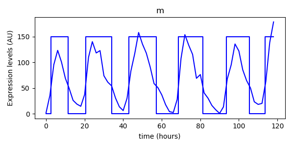
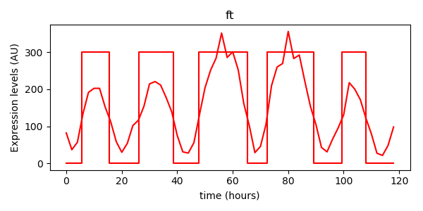
We can plot this over the original data to see how it matches. Note that we rescale the Boolean data purely for display purposes they approximately match the same scale as the experiment data. Remember that the Boolean data only has states True (1) and False (0).

# Now plot the experiment data Boolean time series with the original data

plt.plot(experiment_data[:,2], experiment_data[:,0], 'b-', label="m", )
m_bts.plot(scale=150)
plt.xlabel("time (hours)")
plt.ylabel("Expression levels (AU)")
plt.title("m")
plt.show()


plt.plot(experiment_data[:,2], experiment_data[:,1], 'r-', label="ft")
ft_bts.plot(scale=300)
plt.xlabel("time (hours)")
plt.ylabel("Expression levels (AU)")
plt.title("ft")
plt.show()

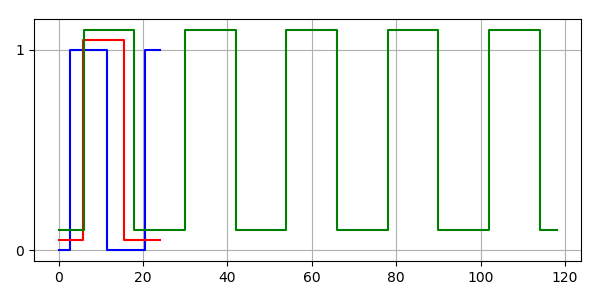
We wish to use the first 24 hours' worth of data as history for our simulation. So we can cut this data to extract the first 24 hours:

# We wish to use the first 24 hours as our history

hist_ft = ft_bts.cut(0, 24)
hist_m = m_bts.cut(0, 24)

# Plot the history
BooleanTimeSeries.plot_many([hist_m, hist_ft])
plt.xlabel("Time (hours)")
plt.legend()
plt.show()

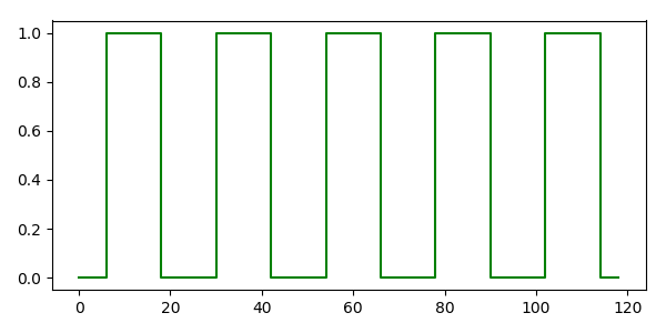
The Circadian model uses light as an input so we need to prepare the light input:

# The model uses a forcing input for light

light_t = [0] + list(range(6,120,12))
light_y = []
for t in light_t:
    light_y.append(6 <= t % 24 < 18)
light_bts = BooleanTimeSeries(light_t, light_y, 118)
light_bts.label = "light"
light_bts.style = "-g"

# Plot light
light_bts.plot()
plt.show()

So the inputs to our simulation are can be plotted on one graph.

# Plot light and the histories
BooleanTimeSeries.plot_many([hist_m, hist_ft, light_bts])
plt.show()

Now we have to define our Boolean Delay Equation model. The model has two simulated states (ft and m) and one input state (light). The model has three delays.

def neurospora_eqns(z, forced_inputs):
    m = 0
    ft = 1
    light = 0
    tau1 = 0
    tau2 = 1
    tau3 = 2

    return [ (not z[tau2][ft]) or forced_inputs[tau3][light], z[tau1][m] ]

For given values of the delays (determined by parameter fitting algorithms such as pynmmso) we can run the simulation for 118 hours:

# Run the simulator

tau1 = 5.0752
tau2 = 6.0211
tau3 = 14.5586
delays = [tau1, tau2, tau3]

solver = BDESolver(neurospora_eqns, delays, [hist_m, hist_ft], [light_bts])
[m_output, ft_output] = solver.solve(118)

We can now plot the output of the simulation:

plt.title("Simulation output")
BooleanTimeSeries.plot_many([m_output , ft_output, light_bts])
plt.xlabel("Time (hours)")
plt.legend()
plt.show()

Plotting these outputs over the original experiment data:

plt.plot(experiment_data[:,2], experiment_data[:,0], 'b-', label="m", )
m_output.plot(scale=150)
plt.xlabel("time (hours)")
plt.ylabel("Expression levels (AU)")
plt.title("m")
plt.show()


plt.plot(experiment_data[:,2], experiment_data[:,1], 'r-', label="ft")
ft_output.plot(scale=300)
plt.xlabel("time (hours)")
plt.ylabel("Expression levels (AU)")
plt.title("ft")
plt.show()

Plotting the simulated data alongside the thresholded data gives:

# Plot simulated data alongside thresholded data

m_output.label = "m sim"
m_output.style = 'c-'
BooleanTimeSeries.plot_many([m_bts, m_output])
plt.xlabel("time (hours)")
plt.title("m")
plt.legend()
plt.show()

ft_output.label = "ft sim"
ft_output.style = 'c-'
BooleanTimeSeries.plot_many([ft_bts, ft_output])
plt.xlabel("time (hours)")
plt.title("ft")
plt.legend()
plt.show()

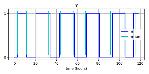
We can calculate the Hamming distance which gives a measure of what duration of time two Boolean time series have differing signals. For 96 hours of simulated time the Hamming distance measures are low:

# Calculate Hamming distances

print("Hamming of m : {:.4f}".format(m_bts.hamming_distance(m_output)))
print("Hamming of ft : {:.4f}".format(ft_bts.hamming_distance(ft_output)))

print("Hamming of m as %age of simulated time: {:.2f}%".format(
    m_bts.hamming_distance(m_output)/0.96))
print("Hamming of ft as %age of simulated time : {:.2f}%".format(
    ft_bts.hamming_distance(ft_output)/0.96))

Which outputs:

Hamming of m : 9.3353
Hamming of ft : 14.7796
Hamming of m as %age of simulated time: 9.72%
Hamming of ft as %age of simulated time : 15.40%

Using pybde with pynmmso

In the above real world example the delay values were explicitly given. In practice they often be obtained as the results of a parameter optimisation exercise. Here we show how to use pynmmso can be used to determine the values of the delays that result in the best fit to the experiment data.

This code follows on from the above real world example. The details of pynmmso are explained in the pynmmso documentation. It is important to know that pynmmso seeks to maximise a fitness function and returns multiple maxima at peaks of the fitness landscape rather then simply the global maximum.

Define our problem class that provides the fitness function and the parameter bounds:

class MyProblem:
    def __init__(self, equations, history, inputs, experiment_data):
        self.equations = equations
        self.history = history
        self.inputs = inputs
        self.experiment_data = experiment_data
        
    def fitness(self, delays):
        # Simulate with the given delay parameters
        solver = BDESolver(self.equations, delays, self.history, self.inputs)
        [m_output, ft_output] = solver.solve(118)
        
        # Compare the result with the Boolean version of the experiment data
        cost = m_output.hamming_distance(self.experiment_data[0]) + ft_output.hamming_distance(self.experiment_data[1])
        
        # Because pynmmso looks for maxima we negate the cost so it looks for the smallest
        # cost
        return -cost
        
    def get_bounds(self):
        # For each of the three delay values explore the range 1..20
        return [1, 1, 1],[20,20,20]

Now use pynmmso to find the maxima:

number_of_fitness_evaluations = 50000

nmmso = Nmmso(MyProblem(neurospora_eqns, [hist_m, hist_ft], [light_bts], [m_bts, ft_bts]))
my_result = nmmso.run(number_of_fitness_evaluations)
for mode_result in my_result:
    print("Mode at {} has value {}".format(mode_result.location, mode_result.value))

This will produce output similar to the following although the actual values returned may be slightly different:

Mode at [ 9.99999999 19.99999998 15.17078072] has value -48.860801508507805
Mode at [19.99999996  7.27463383 15.46914558] has value -73.18395433102842
Mode at [ 5.64100973  7.90184814 13.70187647] has value -19.722341133743335
Mode at [19.95614228  3.5720228   1.03870254] has value -90.91490635269514
Mode at [20.         11.40358844 16.59000251] has value -74.00207006980949
Mode at [19.99915781 15.64418847 15.86933091] has value -75.92303065045431
Mode at [19.99998653 19.44037368  1.07194677] has value -95.11612551719436
Mode at [19.99999884  9.72558647  1.00212142] has value -86.6759957429595
Mode at [20.         11.40358844 18.00923951] has value -74.00207006980948
Mode at [19.87677477  3.40047693 18.00923951] has value -76.36160166053793
Mode at [19.87677477  3.40047693 16.94265386] has value -75.85875891998987
Mode at [ 4.45554284 19.27618803 16.02055511] has value -50.81186043628735
Mode at [1.00000066 4.99999932 1.        ] has value -83.91461625103807
Mode at [ 5.3953705   4.27897001 15.24473766] has value -18.939534918789544

The two solutions with a value of -18.9 and -19.7 look primising and have a lower combined Hamming distance score than the parameters originally used in the example above.

Acknowledgements

This work was supported by the Engineering and Physical Sciences Research Council (grant number EP/N018125/1)