import numpy
from spherical_kde import SphericalKDE
import matplotlib.pyplot as plt
import cartopy.crs
from matplotlib.gridspec import GridSpec, GridSpecFromSubplotSpec

# Choose a seed for deterministic plot
numpy.random.seed(seed=0)

# Set up a grid of figures
fig = plt.figure(figsize=(10, 10))
gs_vert = GridSpec(3, 1)
gs_lower = GridSpecFromSubplotSpec(1, 2, subplot_spec=gs_vert[1])

fig.add_subplot(gs_vert[0], projection=cartopy.crs.Mollweide())
fig.add_subplot(gs_lower[0], projection=cartopy.crs.Orthographic())
fig.add_subplot(gs_lower[1], projection=cartopy.crs.Orthographic(-10, 45))
fig.add_subplot(gs_vert[2], projection=cartopy.crs.PlateCarree())

# Choose parameters for samples
nsamples = 100
pi = numpy.pi

# Generate some samples centered on (1,1) +/- 0.3 radians
theta_samples = numpy.random.normal(loc=1, scale=0.3, size=nsamples)
phi_samples = numpy.random.normal(loc=1, scale=0.3, size=nsamples)
phi_samples = numpy.mod(phi_samples, pi*2)
kde_green = SphericalKDE(phi_samples, theta_samples)

# Generate some samples centered on (-1,1) +/- 0.4 radians
theta_samples = numpy.random.normal(loc=1, scale=0.4, size=nsamples)
phi_samples = numpy.random.normal(loc=-1, scale=0.4, size=nsamples)
phi_samples = numpy.mod(phi_samples, pi*2)
kde_red = SphericalKDE(phi_samples, theta_samples)

# Generate a spread of samples along latitude 2, height 0.1
theta_samples = numpy.random.normal(loc=2, scale=0.1, size=nsamples)
phi_samples = numpy.random.uniform(low=-pi/2, high=pi/2, size=nsamples)
phi_samples = numpy.mod(phi_samples, pi*2)
kde_blue = SphericalKDE(phi_samples, theta_samples, bandwidth=0.1)

for ax in fig.axes:
    ax.set_global()
    ax.gridlines()
    ax.coastlines(linewidth=0.1)
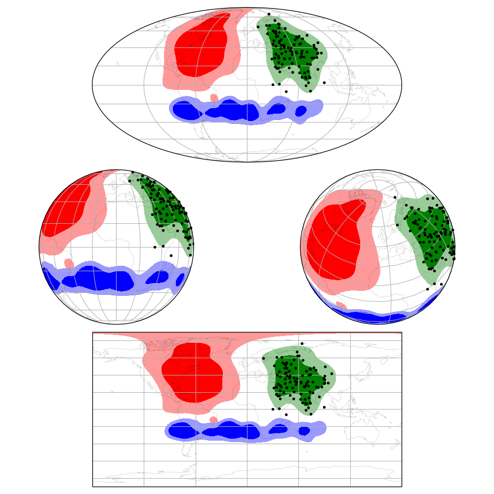
    kde_green.plot(ax, 'g')
    kde_green.plot_samples(ax)
    kde_red.plot(ax, 'r')
    kde_blue.plot(ax, 'b')

# Save to plot
fig.tight_layout()
fig.savefig('plot.png')