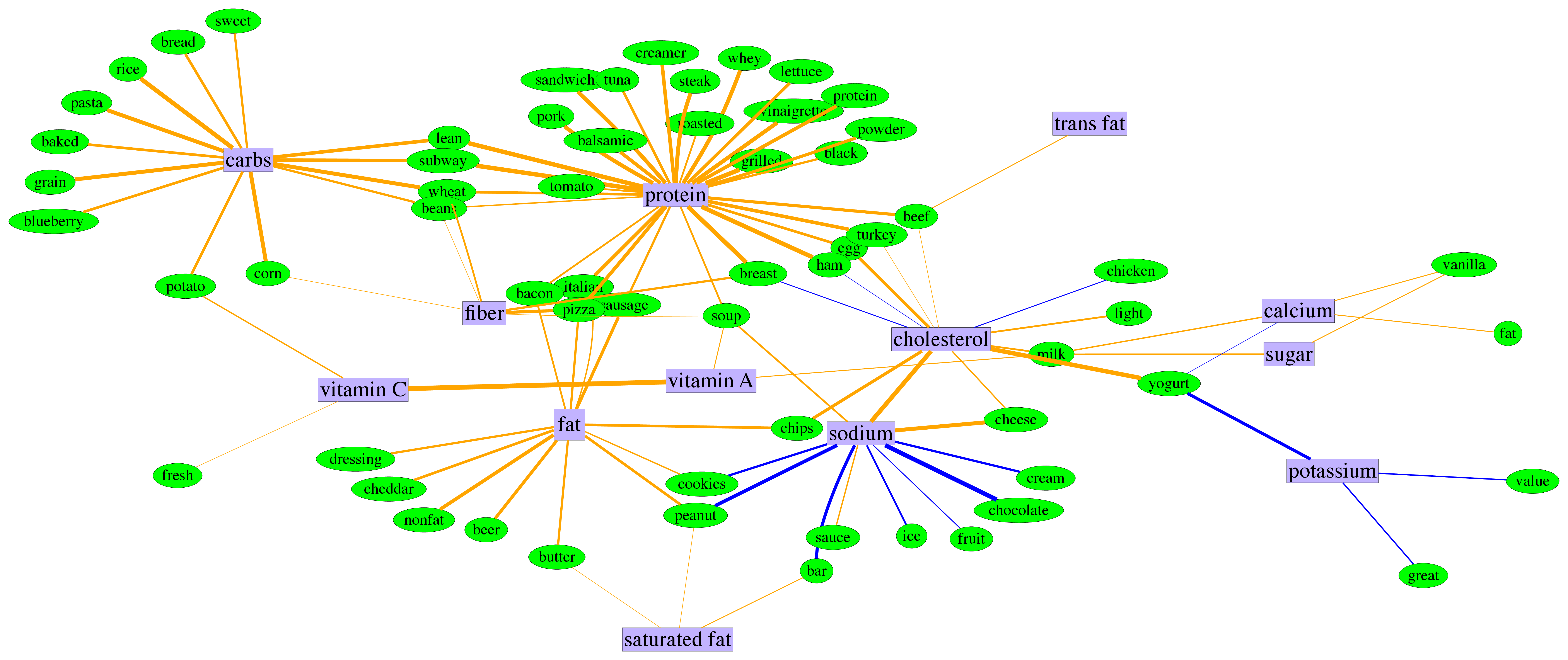
Vector-Space Markov Random Fields
This package provides support for learning MRFs where each node-conditional can be any generic exponential family distribution. Currently supported node-conditionals are Bernoulli, Gamma, Gaussian, Dirichlet, and Point-Inflated models. See exponential_families.py for guidance on how to add a custom node-conditional distribution.
Installation
pip install vsmrfs
Requires numpy, scipy, and matplotlib.
Running
0) Experiment directory structure
The vsmrfs package is very opinionated. It assumes you have an experiment directory with a very specific structure. If your experiment directory is exp, then you need the following structure:
exp/
    args/
    data/
        nodes.csv
        sufficient_statistics.csv
    edges/
    metrics/
    plots/
    weights/
Note that all you really need at first is the exp/data/ structure and the two files. If you generate your data from the synthetic dataset creator, the structure will be created for you.
1a) Generating synthetic data (optional)
If you are just trying to run the package or conduct some benchmarks on the algorithm, you can create a synthetic dataset which will setup all of the experiment structure for you. For example, say you wanted to run an experiment with two Bernoulli nodes and a three-dimensional Dirichlet node, and you want to use foo/ as your experiment directory:
vsmrf-gen foo --nodes b b d3
This will generate a foo directory and all of the structure from step 0, using some default parameters for sparsity and sample sizes. You can see the full list of options with vsmrf-gen --help.
1b) Preparing your data (alternative to 1a)
If you actually have some data that you're trying to model, you need to get it into the right format. Assuming you know your data types, and your experiment directory is foo, you need to generate two files:
foo/data/nodes.csv: This is a single-line CSV file containing the data-types of all your node-conditionals. Currently supported options:
-
b: Bernoulli node -
n: Normal or Gaussian node -
g: Gamma node -
d#: Dirichlet node, where # is replaced with the dimensionality of the Dirichlet, e.g.d3for a 3-parameter Dirichlet -
ziX: Zero-inflated or generic point-inflated node, whereXis replaced by the inflated distribution. This is a recursive definition, so you can have multiple inflated points, e.g.,zizigwould be a two-point inflated Gamma distribution.
foo/data/sufficient_statistics.csv: A CSV matrix of sufficient statistics for all of the node-conditionals. The first line should be the column-to-node-ID mapping. So for example if you have a dataset of two Bernoulli nodes and a 3-dimensional Dirichlet, your header would look like 0,1,2,2,2 since node0 and node1 are both Bernoulli (i.e. univariate sufficient statistics) and node2 is your Dirichlet, with 3 sufficient statistics. Every subsequent row in the file then corresponds to a data sample.
2) MLE via Pseudo-likelihood
To learn a VS-MRF, we make a pseudo-likelihood approximation that effectively decouples all the nodes. This makes the problem convex and separable, enabling us to learn each node independently. If you have access to a cluster or distributed compute environment, this makes the process very fast since you can learn each node on a different machine, then stitch the whole graph back together in step 3.
Say you want to learn the Dirichlet node from step 2, using a solution path approach so you can avoid hyperparameter setting:
vsmrf-learn foo --target 2 --solution_path
This will load the data from the foo experiment directory and learn the pseudo-edges for node2, which is our Dirichlet node. You can see the full list of options with vsmrf-learn --help.
3) Stitching the MRF together
Once all the nodes have been learned, the pseudo-edges need to be combined back together to form a single graph. Since we are learning approximate models, there will be times when a pseudo-edge for nodeA-nodeB exists but nodeB-nodeA does not. In that case, we have to decide whether to include the edge in the final graph or not; that is, should we OR the edges together or AND them? The package will create both, but empirically it seems performance is slightly better with the AND graph.
Continuing our example, to stitch together our three node MRF:
vsmrf-stitch foo --nodes b b d3
If you generated your data synthetically, such that you know the ground truth of the model, you can evaluate the resulting graph:
vsmrf-stitch foo --nodes b b d3 --evaluate
See vsmrf-stitch --help for a full list of options.
Reference
@inproceedings{tansey:etal:2015,
  title={Vector-Space Markov Random Fields via Exponential Families},
  author={Tansey, Wesley and Madrid-Padilla, Oscar H and Suggala, Arun and Ravikumar, Pradeep},
  booktitle={Proceedings of the 32nd International Conference on Machine Learning (ICML-15)},
  year={2015}
}
